In this recipe, we will perform the training and deployment steps in Amazon Sagemaker using the custom container image we pushed to the ECR repository in the Pushing the custom Python algorithm container image to an Amazon ECR repository recipe. In Chapter 1, Getting Started with Machine Learning Using Amazon SageMaker, we used the image URI of the container image of the built-in Linear Learner. In this chapter, we will use the image URI of the custom container image instead.
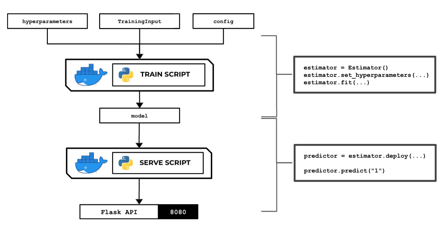
The following diagram shows how SageMaker passes data, files, and configuration to and from each custom container when we use the fit() and predict() functions with the SageMaker Python SDK:
Figure 2.70 – The train and serve scripts inside the custom container make use of the hyperparameters, input data, and config specified using the SageMaker Python SDK
We will also take a look at how to use local mode in this recipe. This capability of SageMaker allows us to test and emulate the CPU and GPU training jobs inside our local environment. Using local mode is useful while we are developing, enhancing, and testing our custom algorithm container images and scripts. We can easily switch to using ML instances that support the training and deployment steps once we are ready to roll out the stable version of our container image.
Once we have completed this recipe, we will be able to run training jobs and deploy inference endpoints using Python with custom train and serve scripts inside custom containers.
Getting ready
Here are the prerequisites for this recipe:
- This recipe continues from the Pushing the custom Python algorithm container image to an Amazon ECR repository recipe.
- We will use the SageMaker Notebook instance from the Launching an Amazon SageMaker Notebook instance and preparing the prerequisites recipe of Chapter 1, Getting Started with Machine Learning Using Amazon SageMaker.
How to do it…
The first couple of steps in this recipe focus on preparing the Jupyter Notebook using the conda_python3 kernel:
- Inside your SageMaker Notebook instance, create a new directory called
chapter02 inside the my-experiments directory. As shown in the following screenshot, we can perform this step by clicking the New button and then choosing Folder (under Other):Figure 2.71 – New > Folder
This will create a directory named Untitled Folder.
- Click the checkbox and then click Rename. Change the name to
chapter02:Figure 2.72 – Renaming "Untitled Folder" to "chapter02"
After that, we should get the desired directory structure, as shown in the preceding screenshot. Now, let's look at the following directory structure:
Figure 2.73 – Directory structure
This screenshot shows how we want to organize our files and notebooks. As we go through each chapter, we will add more directories using the same naming convention to keep things organized.
- Click the chapter02 directory to navigate to /my-experiments/chapter02.
- Create a new notebook by clicking New and then clicking conda_python3:
Figure 2.74 – Creating a new notebook using the conda_python3 kernel
Now that we have a fresh Jupyter Notebook using the conda_python3 kernel, we will proceed with preparing the prerequisites for the training and deployment steps.
- In the first cell of the Jupyter Notebook, use
pip install to upgrade sagemaker[local]:!pip install 'sagemaker[local]' --upgrade
This will allow us to use local mode. We can use local mode when working with framework images such as TensorFlow, PyTorch, scikit-learn, and MXNet, and custom images we have built ourselves.
Important note
Note that we can NOT use local mode in SageMaker Studio. We also can NOT use local mode with built-in algorithms.
- Specify the bucket name where the
training_data.csv file is stored. Use the bucket name we created in the Preparing the Amazon S3 bucket and the training dataset for the linear regression experiment recipe of Chapter 1, Getting Started with Machine Learning Using Amazon SageMaker:s3_bucket = "<insert bucket name here>"
prefix = "chapter01"
Note that our training_data.csv file should exist already inside the S3 bucket and should have the following path:
s3://<S3 BUCKET NAME>/<PREFIX>/input/training_data.csv
- Set the variable values for
training_s3_input_location and training_s3_output_location:training_s3_input_location = \ f"s3://{s3_bucket}/{prefix}/input/training_data.csv"
training_s3_output_location = \ f"s3://{s3_bucket}/{prefix}/output/custom/"
- Import the SageMaker Python SDK and check its version:
import sagemaker
sagemaker.__version__
We should get a value equal to or near 2.31.0 after running the previous block of code.
- Set the value of the container image. Use the value from the Pushing the custom Python algorithm container image to an Amazon ECR repository recipe. The
container variable should be set to a value similar to <ACCOUNT_ID>.dkr.ecr.us-east-1.amazonaws.com/chap02_python:1. Make sure to replace <ACCOUNT_ID> with your AWS account ID:container="<insert image uri and tag here>"
To get the value of <ACCOUNT_ID>, run ACCOUNT_ID=$(aws sts get-caller-identity | jq -r ".Account") and then echo $ACCOUNT_ID inside a Terminal. Remember that we performed this step in the Pushing the custom Python algorithm container image to an Amazon ECR repository recipe, so you should get the same value for ACCOUNT_ID.
- Import a few prerequisites such as
role and session. You will probably notice one of the major differences between this recipe and the recipes in Chapter 1, Getting Started with Machine Learning Using Amazon SageMaker – the usage of LocalSession. The LocalSession class allows us to use local mode in the training and deployment steps:import boto3
from sagemaker import get_execution_role
role = get_execution_role()
from sagemaker.local import LocalSession
session = LocalSession()
session.config = {'local': {'local_code': True}}
- Initialize the
TrainingInput object for the train data channel:from sagemaker.inputs import TrainingInput
train = TrainingInput(training_s3_input_location, content_type="text/csv")
Now that we have the prerequisites, we will proceed with initializing Estimator and using the fit() and predict() functions.
- Initialize
Estimator and use container, role, session, and training_s3_output_location as the parameter values when initializing the Estimator object:estimator = sagemaker.estimator.Estimator(
container,
role,
instance_count=1,
instance_type='local',
output_path=training_s3_output_location,
sagemaker_session=session)
Here, we set the instance_type value to local and the sagemaker_session value to session (which is a LocalSession object). This means that when we run the fit() function later, the training job is performed locally and no ML instances will be provisioned for the training job.
Important note
If we want to perform the training job in a dedicated ML instance, simply replace the instance_type value with ml.m5.xlarge (or an alternative ML instance type) and the sagemaker_session value with a Session object. To make sure that we do not encounter training job name validation issues (as we used an underscore in the ECR repository name), specify the base_job_name parameter value with the appropriate value when initializing Estimator.
- Set a few dummy hyperparameters by using the
set_hyperparameters() function. Behind the scenes, these values will passed to the hyperparameters.json file inside the /opt/ml/input/config directory, which will be loaded and used by the train script when we run the fit() function later:estimator.set_hyperparameters(a=1, b=2, c=3)
- Start the training job using
fit():estimator.fit({'train': train})This should generate a set of logs similar to the following:
Figure 2.75 – Using fit() with local mode
Here, we can see a similar set of logs are generated when we run the train script inside our experimentation environment. As with the Training your first model in Python recipe of Chapter 1, Getting Started with Machine Learning Using Amazon SageMaker, the fit() command will prepare an instance for the duration of the training job to train the model. In this recipe, we are using local mode, so no instances are created.
Important note
To compare this to what we did in Chapter 1, Getting Started with Machine Learning Using Amazon SageMaker, we used the fit() function with the Model class from Chapter 1, while we used the fit() function with the Estimator class in this chapter. We can technically use either of these but in this recipe, we went straight ahead and used the fit() function after the Estimator object was initialized, without initializing a separate Model object.
- Use the
deploy() function to deploy the inference endpoint:predictor = estimator.deploy(
initial_instance_count=1,
instance_type='local',
endpoint_name="custom-local-py-endpoint")
As we are using local mode, no instances are created and the container is run inside the SageMaker Notebook instance:
Figure 2.76 – Using deploy() with local mode
As we can see, we are getting log messages in a similar way to how we got them in the Building and testing the custom Python algorithm container image recipe. This means that if we couldn't get the container running in that recipe, then we will not get the container running in this recipe either.
- Once the endpoint is ready, we can use the
predict() function to test if the inference endpoint is working as expected. This will trigger the /invocations endpoint behind the scenes and pass a value of "1" in the POST body:predictor.predict("1")This should yield a set of logs similar to the following:
Figure 2.77 – Using predict() with local mode
Here, we can see the logs from the API web server that was launched by the serve script inside the container. We should get a value similar or close to '881.3428400857507'. We will get the return value of the sample invocations endpoint we have coded in a previous recipe:
@app.route("/invocations", methods=["POST"])
def predict():
    model = load_model()
    ...
    return Response(..., status=200)
If we go back and check the Preparing and testing the serve script in Python recipe in this chapter, we will see that we have full control of how the invocations endpoint works by modifying the code inside the predict() function in the serve script. We have copied a certain portion of the function in the preceding code block for your convenience.
- Use
delete_endpoint() to delete the local prediction endpoint:predictor.delete_endpoint()
We should get a message similar to the following:
Figure 2.78 – Using delete_endpoint() with local mode
As we can see, using delete_endpoint() will result in the Gracefully stopping… message. Given that we are using local mode in this recipe, the delete_endpoint() function will stop the running API server in the SageMaker Notebook instance. If local mode is not used, the SageMaker inference endpoint and the ML compute instance(s) that support it will be deleted.
Now, let's check how this works!
How it works…
In this recipe, we used the custom container image we prepared in the previous sections while training and deploying Python, instead of the built-in algorithms of SageMaker. All the steps are similar to the ones we followed for the built-in algorithms; the only changes you will need to take note of are the container image, the input parameters, and the hyperparameters.
Take note that we have full control of the hyperparameters we can specify in Estimator as this depends on the hyperparameters that are expected by our custom script. If you need a more realistic example of these hyperparameters, here are the hyperparameters from Chapter 1, Getting Started with Machine Learning Using Amazon SageMaker:
estimator.set_hyperparameters(
    predictor_type='regressor',
    mini_batch_size=4)
In this example, the hyperparameters.json file, which contains the following content, is created when the fit() function is called:
{"predictor_type": "regressor", "mini_batch_size": 4}
The arguments we can use and configure in this recipe are more or less the same as the ones we used for the built-in algorithms of SageMaker. The only major difference is that we are using the container image URI of our ECR repository instead of the container image URI for the built-in algorithms.
When we're using our custom container images, we have the option to use local mode when performing training and deployment. With local mode, no additional instances outside of the SageMaker Notebook instance are created. This allows us to test if the custom container image is working or not, without having to wait for a couple of minutes compared to using real instances (for example, ml.m5.xlarge). Once things are working as expected using local mode, we can easily switch to using the real instances by replacing session and instance_type in Estimator.


 Free Chapter