Sign In Start Free Trial
Account

Add to playlist

Create a Playlist

Modal Close icon
You need to login to use this feature.
  • Book Overview & Buying Python for Finance
  • Table Of Contents Toc
  • Feedback & Rating feedback
Python for Finance

Python for Finance

3.5 (33)
close
close
Python for Finance

Python for Finance

3.5 (33)

Overview of this book

This book uses Python as its computational tool. Since Python is free, any school or organization can download and use it. This book is organized according to various finance subjects. In other words, the first edition focuses more on Python, while the second edition is truly trying to apply Python to finance. The book starts by explaining topics exclusively related to Python. Then we deal with critical parts of Python, explaining concepts such as time value of money stock and bond evaluations, capital asset pricing model, multi-factor models, time series analysis, portfolio theory, options and futures. This book will help us to learn or review the basics of quantitative finance and apply Python to solve various problems, such as estimating IBM’s market risk, running a Fama-French 3-factor, 5-factor, or Fama-French-Carhart 4 factor model, estimating the VaR of a 5-stock portfolio, estimating the optimal portfolio, and constructing the efficient frontier for a 20-stock portfolio with real-world stock, and with Monte Carlo Simulation. Later, we will also learn how to replicate the famous Black-Scholes-Merton option model and how to price exotic options such as the average price call option.
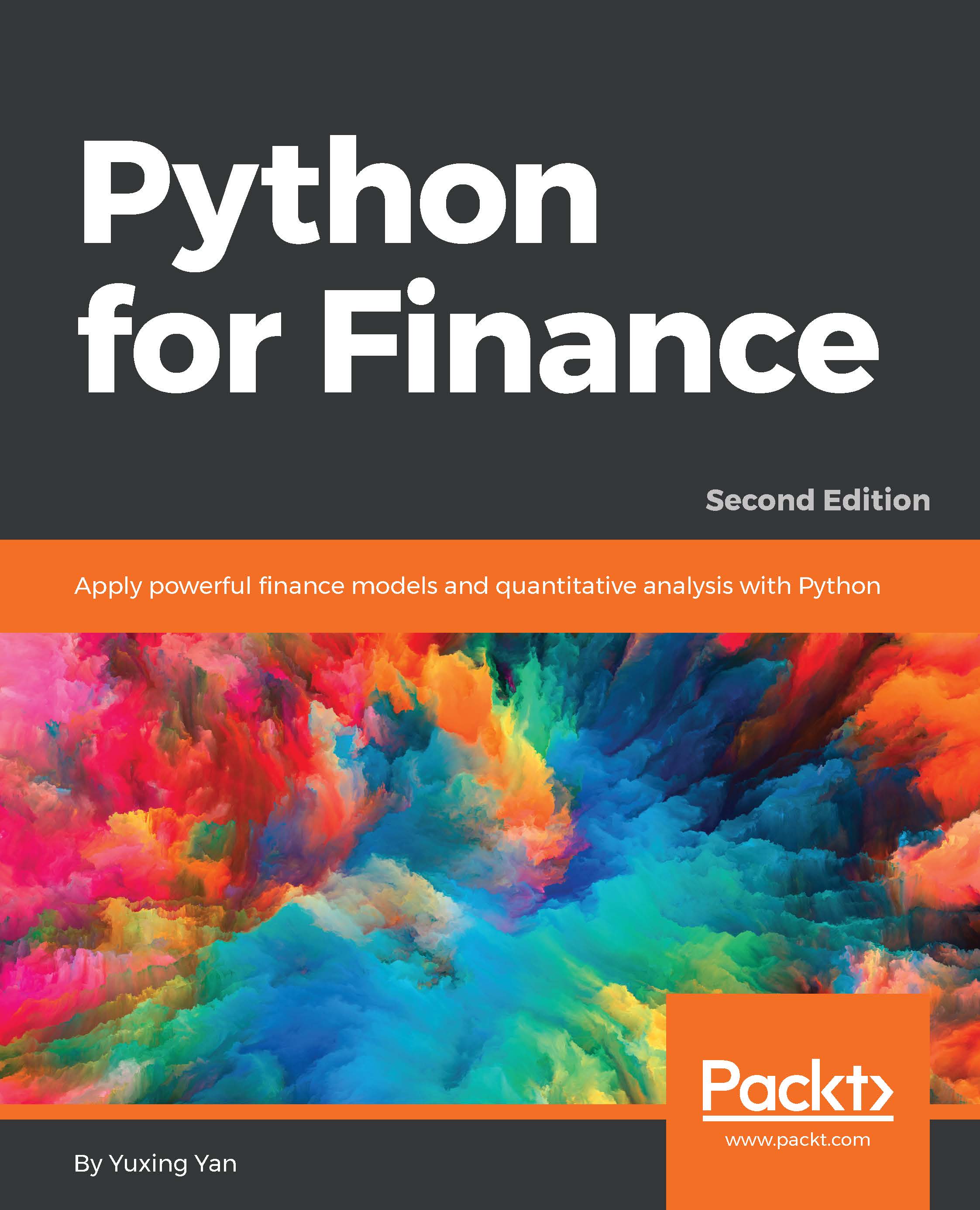
Table of Contents (17 chapters)
close
close
16
Index

Understanding the interpolation technique

Interpolation is a technique used quite frequently in finance. In the following example, we have to replace two missing values, NaN, between 2 and 6. The pandas.interpolate() function, for a linear interpolation, is used to fill in the two missing values:

import pandas as pd 
import numpy as np 
nn=np.nan
x=pd.Series([1,2,nn,nn,6]) 
print(x.interpolate())

The output is shown here:

0    1.000000
1    2.000000
2    3.333333
3    4.666667
4    6.000000
dtype: float64

The preceding method is a linear interpolation. Actually, we could estimate a Δ and calculate those missing values manually:

Understanding the interpolation technique

Here, v2(v1) is the second (first) value and n is the number of intervals between those two values. For the preceding case, Δ is (6-2)/3=1.33333. Thus, the next value will be v1+Δ=2+1.33333=3.33333. This way, we could continually estimate all missing values. Note that if we have several periods with missing values, then the delta for each period has...

Unlock full access

Continue reading for free

A Packt free trial gives you instant online access to our library of over 7000 practical eBooks and videos, constantly updated with the latest in tech
bookmark search playlist font-size

Change the font size

margin-width

Change margin width

day-mode

Change background colour

Close icon Search
Country selected

Close icon Your notes and bookmarks

Delete Bookmark

Modal Close icon
Are you sure you want to delete it?
Cancel
Yes, Delete

Confirmation

Modal Close icon
claim successful

Buy this book with your credits?

Modal Close icon
Are you sure you want to buy this book with one of your credits?
Close
YES, BUY