Chapter 3: Introduction to Machine Learning via Scikit-Learn
Activity 5: Generating Predictions and Evaluating the Performance of a Multiple Linear Regression Model
Solution:
- Generate predictions on the test data using the following:
predictions = model.predict(X_test)
2. Plot the predicted versus actual values on a scatterplot using the following code:
import matplotlib.pyplot as plt
from scipy.stats import pearsonr
plt.scatter(y_test, predictions)
plt.xlabel('Y Test (True Values)')
plt.ylabel('Predicted Values')
plt.title('Predicted vs. Actual Values (r = {0:0.2f})'.format(pearsonr(y_test, predictions)[0], 2))
plt.show()
Refer to the resultant output here:
Figure 3.33: A scatterplot of predicted versus actual values from a multiple linear regression model
Note
There is a much stronger linear correlation between the predicted and actual values in the multiple linear regression model (r = 0.93) relative to the simple linear regression model (r = 0.62).
- To plot the distribution of the residuals, refer to the code here:
import seaborn as sns
from scipy.stats import shapiro
sns.distplot((y_test - predictions), bins = 50)
plt.xlabel('Residuals')
plt.ylabel('Density')
plt.title('Histogram of Residuals (Shapiro W p-value = {0:0.3f})'.format(shapiro(y_test - predictions)[1]))
plt.show()
Refer to the resultant output here:
Figure 3.34: The distribution of the residuals from a multiple linear regression model
Note
Our residuals are negatively skewed and non-normal, but this is less skewed than in the simple linear model.
- Calculate the metrics for mean absolute error, mean squared error, root mean squared error, and R-squared, and put them into a DataFrame as follows:
from sklearn import metrics
import numpy as np
metrics_df = pd.DataFrame({'Metric': ['MAE',
'MSE',
'RMSE',
'R-Squared'],
'Value': [metrics.mean_absolute_error(y_test, predictions),
metrics.mean_squared_error(y_test, predictions),
np.sqrt(metrics.mean_squared_error(y_test, predictions)),
metrics.explained_variance_score(y_test, predictions)]}).round(3)
print(metrics_df)
Please refer to the resultant output:
Figure 3.35: Model evaluation metrics from a multiple linear regression model
The multiple linear regression model performed better on every metric relative to the simple linear regression model.
Activity 6: Generating Predictions and Evaluating Performance of a Tuned Logistic Regression Model
Solution:
- Generate the predicted probabilities of rain using the following code:
predicted_prob = model.predict_proba(X_test)[:,1]
- Generate the predicted class of rain using predicted_class = model.predict(X_test).
- Evaluate performance using a confusion matrix and save it as a DataFrame using the following code:
from sklearn.metrics import confusion_matrix
import numpy as np
cm = pd.DataFrame(confusion_matrix(y_test, predicted_class))
cm['Total'] = np.sum(cm, axis=1)
cm = cm.append(np.sum(cm, axis=0), ignore_index=True)
cm.columns = ['Predicted No', 'Predicted Yes', 'Total']
cm = cm.set_index([['Actual No', 'Actual Yes', 'Total']])
print(cm)
Figure 3.36: The confusion matrix from our logistic regression grid search model
Note
Nice! We have decreased our number of false positives from 6 to 2. Additionally, our false negatives were lowered from 10 to 4 (see in Exercise 26). Be aware that results may vary slightly.
- For further evaluation, print a classification report as follows:
from sklearn.metrics import classification_report
print(classification_report(y_test, predicted_class))
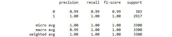
Figure 3.37: The classification report from our logistic regression grid search model
By tuning the hyperparameters of the logistic regression model, we were able to improve upon a logistic regression model that was already performing very well.
Activity 7: Generating Predictions and Evaluating the Performance of the SVC Grid Search Model
Solution:
- Extract predicted classes of rain using the following code:
predicted_class = model.predict(X_test)
- Create and print a confusion matrix using the code here:
from sklearn.metrics import confusion_matrix
import numpy as np
cm = pd.DataFrame(confusion_matrix(y_test, predicted_class))
cm['Total'] = np.sum(cm, axis=1)
cm = cm.append(np.sum(cm, axis=0), ignore_index=True)
cm.columns = ['Predicted No', 'Predicted Yes', 'Total']
cm = cm.set_index([['Actual No', 'Actual Yes', 'Total']])
print(cm)
See the resultant output here:
Figure 3.38: The confusion matrix from our SVC grid search model
- Generate and print a classification report as follows:
from sklearn.metrics import classification_report
print(classification_report(y_test, predicted_class))
See the resultant output here:
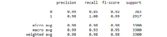
Figure 3.39: The classification report from our SVC grid search model
Here, we demonstrated how to tune the hyperparameters of an SVC model using grid search.
Activity 8: Preparing Data for a Decision Tree Classifier
Solution:
- Import weather.csv and store it as a DataFrame using the following:
import pandas as pd
df = pd.read_csv('weather.csv')
- Dummy code the Description column as follows:
import pandas as pd
df_dummies = pd.get_dummies(df, drop_first=True)
- Shuffle df_dummies using the following code:
from sklearn.utils import shuffle
df_shuffled = shuffle(df_dummies, random_state=42)
- Split df_shuffled into X and y as follows:
DV = 'Rain'
X = df_shuffled.drop(DV, axis=1)
y = df_shuffled[DV]
- Split X and y into testing and training data:
from sklearn.model_selection import train_test_split
X_train, X_test, y_train, y_test = train_test_split(X, y, test_size=0.33, random_state=42)
- Scale X_train and X_test using the following code:
from sklearn.preprocessing import StandardScaler
model = StandardScaler()
X_train_scaled = model.fit_transform(X_train)
X_test_scaled = model.transform(X_test)
Activity 9: Generating Predictions and Evaluating the Performance of a Decision Tree Classifier Model
Solution:
- Generate the predicted probabilities of rain using the following:
predicted_prob = model.predict_proba(X_test_scaled)[:,1]
- Generate the predicted classes of rain using the following:
predicted_class = model.predict(X_test)
- Generate and print a confusion matrix with the code here:
from sklearn.metrics import confusion_matrix
import numpy as np
cm = pd.DataFrame(confusion_matrix(y_test, predicted_class))
cm['Total'] = np.sum(cm, axis=1)
cm = cm.append(np.sum(cm, axis=0), ignore_index=True)
cm.columns = ['Predicted No', 'Predicted Yes', 'Total']
cm = cm.set_index([['Actual No', 'Actual Yes', 'Total']])
print(cm)
Refer to the resultant output here:
Figure 3.40: The confusion matrix from our tuned decision tree classifier model
- Print a classification report as follows:
from sklearn.metrics import classification_report
print(classification_report(y_test, predicted_class))
Refer to the resultant output here:
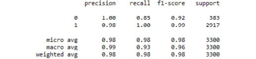
Figure 3.41: The classification report from our tuned decision tree classifier model
There was only one misclassified observation. Thus, by tuning a decision tree classifier model on our weather.csv dataset, we were able to predict rain (or snow) with great accuracy. We can see that the sole driving feature was temperature in Celsius. This makes sense due to the way in which decision trees use recursive partitioning to make predictions.
Activity 10: Tuning a Random Forest Regressor
Solution:
- Specify the hyperparameter space as follows:
import numpy as np
grid = {'criterion': ['mse','mae'],
'max_features': ['auto', 'sqrt', 'log2', None],
'min_impurity_decrease': np.linspace(0.0, 1.0, 10),
'bootstrap': [True, False],
'warm_start': [True, False]}
- Instantiate the GridSearchCV model, optimizing the explained variance using the following code:
from sklearn.model_selection import GridSearchCV
from sklearn.ensemble import RandomForestRegressor
model = GridSearchCV(RandomForestRegressor(), grid, scoring='explained_variance', cv=5)
- Fit the grid search model to the training set using the following (note that this may take a while):
model.fit(X_train_scaled, y_train)
See the output here:
Figure 3.42: The output from our tuned random forest regressor grid search model
- Print the tuned parameters as follows:
best_parameters = model.best_params_
print(best_parameters)
See the resultant output below:
Figure 3.43: The tuned hyperparameters from our random forest regressor grid search model
Activity 11: Generating Predictions and Evaluating the Performance of a Tuned Random Forest Regressor Model
Solution:
- Generate predictions on the test data using the following:
predictions = model.predict(X_test_scaled)
- Plot the correlation of predicted and actual values using the following code:
import matplotlib.pyplot as plt
from scipy.stats import pearsonr
plt.scatter(y_test, predictions)
plt.xlabel('Y Test (True Values)')
plt.ylabel('Predicted Values')
plt.title('Predicted vs. Actual Values (r = {0:0.2f})'.format(pearsonr(y_test, predictions)[0], 2))
plt.show()
Refer to the resultant output here:
Figure 3.44: A scatterplot of predicted and actual values from our random forest regression model with tuned hyperparameters
- Plot the distribution of residuals as follows:
import seaborn as sns
from scipy.stats import shapiro
sns.distplot((y_test - predictions), bins = 50)
plt.xlabel('Residuals')
plt.ylabel('Density')
plt.title('Histogram of Residuals (Shapiro W p-value = {0:0.3f})'.format(shapiro(y_test - predictions)[1]))
plt.show()
Refer to the resultant output here:
Figure 3.45: A histogram of residuals from a random forest regression model with tuned hyperparameters
- Compute metrics, place them in a DataFrame, and print it using the code here:
from sklearn import metrics
import numpy as np
metrics_df = pd.DataFrame({'Metric': ['MAE',
'MSE',
'RMSE',
'R-Squared'],
'Value': [metrics.mean_absolute_error(y_test, predictions),
metrics.mean_squared_error(y_test, predictions),
np.sqrt(metrics.mean_squared_error(y_test, predictions)),
metrics.explained_variance_score(y_test, predictions)]}).round(3)
print(metrics_df)
Find the resultant output here:
Figure 3.46: Model evaluation metrics from our random forest regression model with tuned hyperparameters
The random forest regressor model seems to underperform compared to the multiple linear regression, as evidenced by greater MAE, MSE, and RMSE values, as well as less explained variance. Additionally, there was a weaker correlation between the predicted and actual values, and the residuals were further from being normally distributed. Nevertheless, by leveraging ensemble methods using a random forest regressor, we constructed a model that explains 75.8% of the variance in temperature and predicts temperature in Celsius + 3.781 degrees.


 Free Chapter