

Decision tree learning
This section introduces decision tree learning, a machine learning algorithm essential to understanding LightGBM. We’ll work through an example of how to build decision trees using scikit-learn. This section will also provide some mathematical definitions for building decision trees; understanding these definitions is not critical, but it will help us understand our discussion of the decision tree hyperparameters.
Decision trees are tree-based learners that function by asking successive questions about the data to determine the result. A path is followed down the tree, making decisions about the input using one or more features. The path terminates at a leaf node, which represents the predicted class or value. Decision trees can be used for classification or regression.
The following is an illustration of a decision tree fit on the Iris dataset:
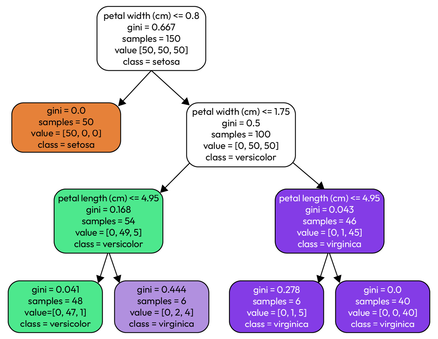
Figure 1.5 – A decision tree modeling the Iris dataset
The Iris dataset is a classification dataset where Iris flower sepal and petal dimensions are used to predict the type of Iris flower. Each non-leaf node uses one or more features to narrow down the samples in the dataset: the root node starts with all 150 samples and then splits them based on petal width, <= 0.8. We continue down the tree, with each node splitting the samples further until we reach a leaf node that contains the predicted class (versicolor, virginica, or setosa).
Compared to other models, decision trees have many advantages:
- Features may be numeric or categorical: Samples can be split using either numerical features (by splitting a range) or categorical ones without us having to encode either.
- Reduced need for data preparation: Decision splits are not sensitive to data ranges or size. Many other models (for example, neural networks) require data to be normalized to unit ranges.
- Interpretability: As shown previously, it’s straightforward to interpret the predictions made by a tree. Interpretability is valuable in contexts where a prediction must be explained to decision-makers.
These are just some of the advantages of using tree-based models. However, we also need to be aware of some of the disadvantages associated with decision trees:
- Overfitting: Decision trees are very prone to overfitting. Setting the correct hyperparameters is essential when fitting decision trees. Overfitting in decision trees will be discussed in detail later.
- Poor extrapolation: Decision trees are poor at extrapolation since their predictions are not continuous and are effectively bounded by the training data.
- Unbalanced data: When fitting a tree on unbalanced data, the high-frequency classes dominate the predictions. Data needs to be prepared to remove imbalances.
A more detailed discussion of the advantages and disadvantages of decision trees is available at https://scikit-learn.org/stable/modules/tree.html.
Entropy and information gain
First, we need a rudimentary understanding of entropy and information gain before we look at an algorithm for building (or fitting) a decision tree.
Entropy can be considered a way to measure the disorder or randomness of a system. Entropy measures how surprising the result of a specific input or event might be. Consider a well-shuffled deck of cards: drawing from the top of the deck could give us any of the cards in the deck (a surprising result each time); therefore, we can say that a shuffled deck of cards has high entropy. Drawing cards from the top of an ordered deck is unsurprising; we know which cards come next. Therefore, an ordered deck of cards has low entropy. Another way to interpret entropy is the impurity of the dataset: a low-entropy dataset (neatly ordered) has less impurity than a high-entropy dataset.
Information gain, in turn, is the amount of information gained when modifying or observing the underlying data. Information gain involves reducing entropy from before the observation. In our deck of cards example, we might take a shuffled deck of cards and split it into four smaller decks by suit (spades, hearts, diamonds, and clubs). If we draw from the smaller decks, the outcome is less of a surprise: we know that the next card is from the same suit. By splitting the deck by suit, we have reduced the entropy of the smaller decks. Splitting the deck of cards on a feature (the suit) is very similar to how the splits in a decision tree work; each division seeks to maximize the information gain – that is, they minimize the entropy after the split.
In decision trees, there are two common ways of measuring information gain or the loss of impurity:
- The Gini index
- Log loss or entropy
A detailed explanation of each is available at https://scikit-learn.org/stable/modules/tree.html#classification-criteria.
Building a decision tree using C4.5
C4.5 is an algorithm for building a decision tree from a dataset [1]. The algorithm is recursive and starts with the following base cases:
- If all the samples in a sub-dataset are of the same class, create a leaf node in the tree that chooses that class.
- If no information can be gained by splitting using any of the features (the dataset can’t be divided any further), create a leaf node that predicts the most frequent class contained in the sub-dataset.
- If a minimum threshold of samples is reached in a sub-dataset, create a leaf node that predicts the most frequent class contained in the sub-dataset.
Then, we can apply the algorithm:
- Check for any of the three base cases and stop splitting if any applies to the dataset.
- For each feature or attribute of the dataset, calculate the information gained by splitting the dataset on that feature.
- Create a decision node by splitting the dataset on the feature with the highest information gain.
- Split the dataset into two sub-datasets based on the decision node and recursively reply to the algorithm on each sub-dataset.
Once the tree has been built, pruning is applied. During pruning, decision nodes with a relatively lower information gain than other tree nodes are removed. Removing nodes avoids overfitting the training data and improves the tree’s generalization ability.
Classification and Regression Tree
You may have noticed that in the preceding explanations, we only used classes to split datasets using decision nodes; this is not by chance, as the canonical C4.5 algorithm only supports classification trees. Classification and Regression Tree (CART) extends C4.5 to support numerical target variables – that is, regression problems [2]. With CART, decision nodes can also split continuous numerical input variables to support regression, typically using a threshold (for example, x <= 0.3). When reaching a leaf node, the mean or median of the remaining numerical range is generally taken as the predicted value.
When building classification trees, only impurity is used to determine splits. However, with regression trees, impurity is combined with other criteria to calculate optimal splits:
- The MSE (or MAE)
- Half Poisson Deviance
A detailed mathematical explanation of each is available at https://scikit-learn.org/stable/modules/tree.html#regression-criteria.
scikit-learn uses an optimized version of CART to build decision trees.
Overfitting in decision trees
One of the most significant disadvantages of decision trees is that they are prone to overfitting. Without proper hyperparameter choices, C4.5 and other training algorithms create overly complex and deep trees that fit the training data almost exactly. Managing overfitting is a crucial part of building decision trees. Here are some strategies to avoid overfitting:
- Pruning: As mentioned previously, we can remove branches that do not contribute much information gain; this reduces the tree’s complexity and improves generalization.
- Maximum depth: Limiting the depth of the tree also avoids overly complex trees and avoids overfitting.
- Maximum number of leaf nodes: Similar to restricting depth, limiting the number of leaf nodes avoids overly specific branches and improves generalization.
- Minimum samples per leaf: Setting a minimum limit on the number of samples a leaf may contain (stopping splitting when the sub-dataset is of the minimum size) also avoids overly specific leaf nodes.
- Ensemble methods: Ensemble learning is a technique that combines multiple models to improve the prediction over an individual model. Averaging the prediction of multiple models can also reduce overfitting.
These strategies can be applied by setting the appropriate hyperparameters. Now that we understand how to build decision trees and strategies for overfitting, let’s look at building decision trees in scikit-learn.
Building decision trees with scikit-learn
It is time to examine how we may use decision trees by training classification and regression trees using scikit-learn.
For these examples, we’ll use the toy datasets included in scikit-learn. These datasets are small compared to real-world data but are easy to work with, allowing us to focus on the decision trees.
Classifying breast cancer
We’ll use the Breast Cancer dataset (https://scikit-learn.org/stable/datasets/toy_dataset.html#breast-cancer-dataset) for our classification example. This dataset consists of features that have been calculated from the images of fine needle aspirated breast masses, and the task is to predict whether the mass is malignant or benign.
Using scikit-learn, we can solve this classification problem with five lines of code:
dataset = datasets.load_breast_cancer()
X_train, X_test, y_train, y_test = train_test_split(dataset.data, dataset.target, random_state=157)
model = DecisionTreeClassifier(random_state=157, max_depth=3, min_samples_split=2)
model = model.fit(X_train, y_train)
f1_score(y_test, model.predict(X_test))
First, we load the dataset using load_breast_cancer. Then, we split our dataset into training and test sets using train_test_split; by default, 25% of the data is used for the test set. Like before, we instantiate our DecisionTreeClassifier model and train it on the training set using model.fit. The two hyperparameters we pass through when instantiating the model are notable: max_depth and min_samples_split. Both parameters control overfitting and will be discussed in more detail in the next section. We also specify random_state for both the train-test split and the model. By fixing the random state, we ensure the outcome is repeatable (otherwise, a new random state is created by scikit-learn for every execution).
Finally, we measure the performance using f1_score. Our model achieves an F1 score of 0.94 and an accuracy of 93.7%. F1 scores are out of 1.0, so we may conclude that the model does very well. If we break down our predictions, the model missed the prediction on only 9 of the 143 samples in the test set: 7 false positives and 2 false negatives.
Predicting diabetes progression
To illustrate solving a regression problem with decision trees, we’ll use the Diabetes dataset (https://scikit-learn.org/stable/datasets/toy_dataset.html#diabetes-dataset). This dataset has 10 features (age, sex, body mass index, and others), and the model is tasked with predicting a quantitative measure of disease progression after 1 year.
We can use the following code to build and evaluate a regression model:
dataset = datasets.load_diabetes()
X_train, X_test, y_train, y_test = train_test_split(dataset.data, dataset.target, random_state=157)
model = DecisionTreeRegressor(random_state=157, max_depth=3, min_samples_split=2)
model = model.fit(X_train, y_train)
mean_absolute_error(y_test, model.predict(X_test))
Our model achieves an MAE of 45.28. The code is almost identical to our classification example: instead of a classifier, we use DecisionTreeRegressor as our model and calculate mean_absolute_error instead of the F1 score. The consistency in the API for solving various problems with different types of models in scikit-learn is by design and illustrates a fundamental truth in machine learning work: even though data, models, and metrics change, the overall process for building machine learning models remains the same. In the coming chapters, we’ll expand on this general methodology and leverage the process’ consistency when building machine learning pipelines.
Decision tree hyperparameters
We used some decision tree hyperparameters in the preceding classification and regression examples to control overfitting. This section will look at the most critical decision tree hyperparameters provided by scikit-learn:
max_depth: The maximum depth the tree is allowed to reach. Deeper trees allow more splits, resulting in more complex trees and overfitting.min_samples_split: The minimum number of samples required to split a node. Nodes containing only a few samples overfit the data, whereas having a larger minimum improves generalization.min_samples_leaf: The minimum number of samples allowed in leaf nodes. Like the minimum samples in a split, increasing the value leads to less complex trees, reducing overfitting.max_leaf_nodes: The maximum number of lead nodes to allow. Fewer leaf nodes reduce the tree size and, therefore, the complexity, which may improve generalization.max_features: The maximum features to consider when determining a split. Discarding some features reduces noise in the data, which improves overfitting. Features are chosen at random.criterion: The impurity measure to use when determining a split, eitherginiorentropy/log_loss.
As you may have noticed, most decision tree hyperparameters involve controlling overfitting by controlling the complexity of the tree. These parameters provide multiple ways of doing so, and finding the best combination of parameters and their values is non-trivial. Finding the best hyperparameters is called hyperparameter tuning and will be covered extensively later in this book.
A complete list of the hyperparameters can be found at the following places:
- https://scikit-learn.org/stable/modules/generated/sklearn.tree.DecisionTreeClassifier.html#sklearn-tree-decisiontreeclassifier
- https://scikit-learn.org/stable/modules/generated/sklearn.tree.DecisionTreeRegressor.html#sklearn.tree.DecisionTreeRegressor
Now, let’s summarize the key takeaways from this chapter.