-
Book Overview & Buying
-
Table Of Contents

-
Feedback & Rating

Julia Programming Projects
By :
Julia Programming Projects
By:
Overview of this book
Julia is a new programming language that offers a unique combination of performance and productivity. Its powerful features, friendly syntax, and speed are attracting a growing number of adopters from Python, R, and Matlab, effectively raising the bar for modern general and scientific computing.
After six years in the making, Julia has reached version 1.0. Now is the perfect time to learn it, due to its large-scale adoption across a wide range of domains, including fintech, biotech, education, and AI.
Beginning with an introduction to the language, Julia Programming Projects goes on to illustrate how to analyze the Iris dataset using DataFrames. You will explore functions and the type system, methods, and multiple dispatch while building a web scraper and a web app. Next, you'll delve into machine learning, where you'll build a books recommender system. You will also see how to apply unsupervised machine learning to perform clustering on the San Francisco business database. After metaprogramming, the final chapters will discuss dates and time, time series analysis, visualization, and forecasting.
We'll close with package development, documenting, testing and benchmarking.
By the end of the book, you will have gained the practical knowledge to build real-world applications in Julia.
Table of Contents (13 chapters)
Preface

 Free Chapter
Getting Started with Julia Programming
Creating Our First Julia App
Setting Up the Wiki Game
Building the Wiki Game Web Crawler
Adding a Web UI for the Wiki Game
Implementing Recommender Systems with Julia
Machine Learning for Recommender Systems
Leveraging Unsupervised Learning Techniques
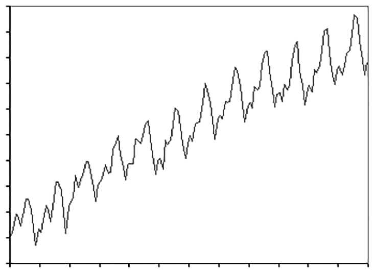
Working with Dates, Times, and Time Series
Time Series Forecasting
Creating Julia Packages
Other Books You May Enjoy
Customer Reviews