Neural networks are a sub-type of machine learning methods that are inspired by the structure and function of the human brain. In neural networks, each computational unit, analogically called a neuron, is connected to other neurons in a layered fashion. When the number of such layers is more than two, the neural network thus formed is called a deep neural network. Such models are generally called deep learning models.
Deep learning models have proven superior to other classical machine learning models because of their ability to learn highly complex relationships between input data and the output (ground truth). In recent times, deep learning has gained a lot of attention and rightly so, primarily because of the following two reasons:
- The availability of powerful computing machines, especially in the cloud
- The availability of huge amounts of data
Owing to Moore's law, which states that the processing power of computers will double every 2 years, we are now living in a time when deep learning models with several hundreds of layers can be trained within a realistic and reasonably short amount of time. At the same time, with the exponential increase in the use of digital devices everywhere, our digital footprint has exploded, resulting in gigantic amounts of data being generated across the world every moment.
Hence, it has been possible to train deep learning models for some of the most difficult cognitive tasks that were either intractable earlier or had sub-optimal solutions through other machine learning techniques.
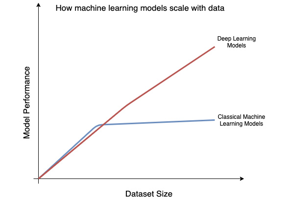
Deep learning, or neural networks in general, has another advantage over the classical machine learning models. Usually, in a classical machine learning-based approach, feature engineering plays a crucial role in the overall performance of a trained model. However, a deep learning model does away with the need to manually craft features. With large amounts of data, deep learning models can perform very well without requiring hand-engineered features and can outperform the traditional machine learning models. The following graph indicates how deep learning models can leverage large amounts of data better than the classical machine models:
Figure 1.2 – Model performance versus dataset size
As can be seen in the graph, deep learning performance isn't necessarily distinguished up to a certain dataset size. However, as the data size starts to further increase, deep neural networks begin outperforming the non-deep learning models.
A deep learning model can be built based on various types of neural network architectures that have been developed over the years. A prime distinguishing factor between the different architectures is the type and combination of layers that are used in the neural network. Some of the well-known layers are the following:
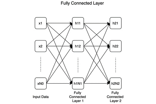
- Fully-connected or linear: In a fully connected layer, as shown in the following diagram, all neurons preceding this layer are connected to all neurons succeeding this layer:
Figure 1.3 – Fully connected layer
This example shows two consecutive fully connected layers with N1 and N2 number of neurons, respectively. Fully connected layers are a fundamental unit of many – in fact, most – deep learning classifiers.
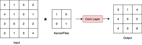
- Convolutional: The following diagram shows a convolutional layer, where a convolutional kernel (or filter) is convolved over the input:
Figure 1.4 – Convolutional layer
Convolutional layers are a fundamental unit of convolutional neural networks (CNNs), which are the most effective models for solving computer vision problems.
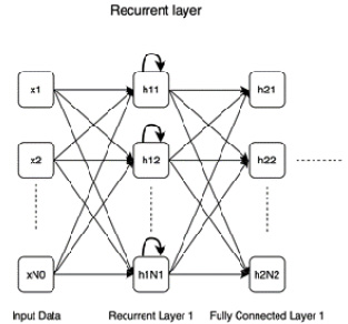
- Recurrent: The following diagram shows a recurrent layer. While it looks similar to a fully connected layer, the key difference is the recurrent connection (marked with bold curved arrows):
Figure 1.5 – Recurrent layer
Recurrent layers have an advantage over fully connected layers in that they exhibit memorizing capabilities, which comes in handy working with sequential data where one needs to remember past inputs along with the present inputs.
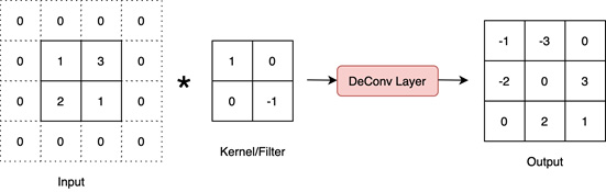
- DeConv (the reverse of a convolutional layer): Quite the opposite of a convolutional layer, a deconvolutional layer works as shown in the following diagram:
Figure 1.6 – Deconvolutional layer
This layer expands the input data spatially and hence is crucial in models that aim to generate or reconstruct images, for example.
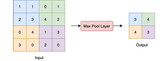
- Pooling: The following diagram shows the max-pooling layer, which is perhaps the most widely used kind of pooling layer:
Figure 1.7 – Pooling layer
This is a max-pooling layer that pools the highest number each from 2x2 sized subsections of the input. Other forms of pooling are min-pooling and mean-pooling.
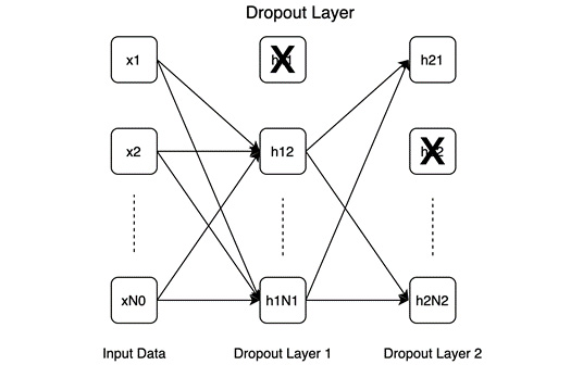
- Dropout: The following diagram shows how dropout layers work. Essentially, in a dropout layer, some neurons are temporarily switched off (marked with X in the diagram), that is, they are disconnected from the network:
Figure 1.8 – Dropout layer
Dropout helps in model regularization as it forces the model to function well in sporadic absences of certain neurons, which forces the model to learn generalizable patterns instead of memorizing the entire training dataset.
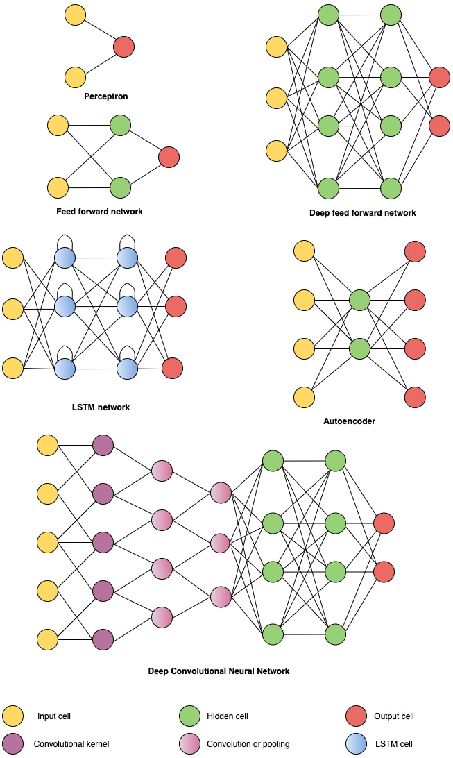
A number of well-known architectures based on the previously mentioned layers are shown in the following diagram:.
Figure 1.9 – Different neural network architectures
A more exhaustive set of neural network architectures can be found here: https://www.asimovinstitute.org/neural-network-zoo/.
Besides the types of layers and how they are connected in a network, other factors such as activation functions and the optimization schedule also define the model.
Activation functions
Activation functions are crucial to neural networks as they add the non-linearity without which, no matter how many layers we add, the entire neural network would be reduced to a simple linear model. The different types of activation functions listed here are basically different nonlinear mathematical functions.
Some of the popular activation functions are as follows:
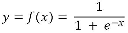
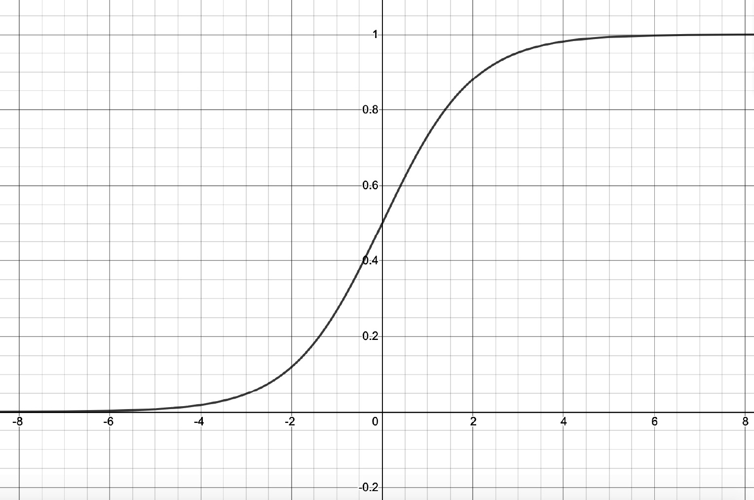
- Sigmoid: A sigmoid (or logistic) function is expressed as follows:
The function is shown in graph form as follows:
Figure 1.10 – Sigmoid function
As can be seen from the graph, the sigmoid function takes in a numerical value x as input and outputs a value y in the range (0, 1).
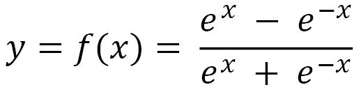
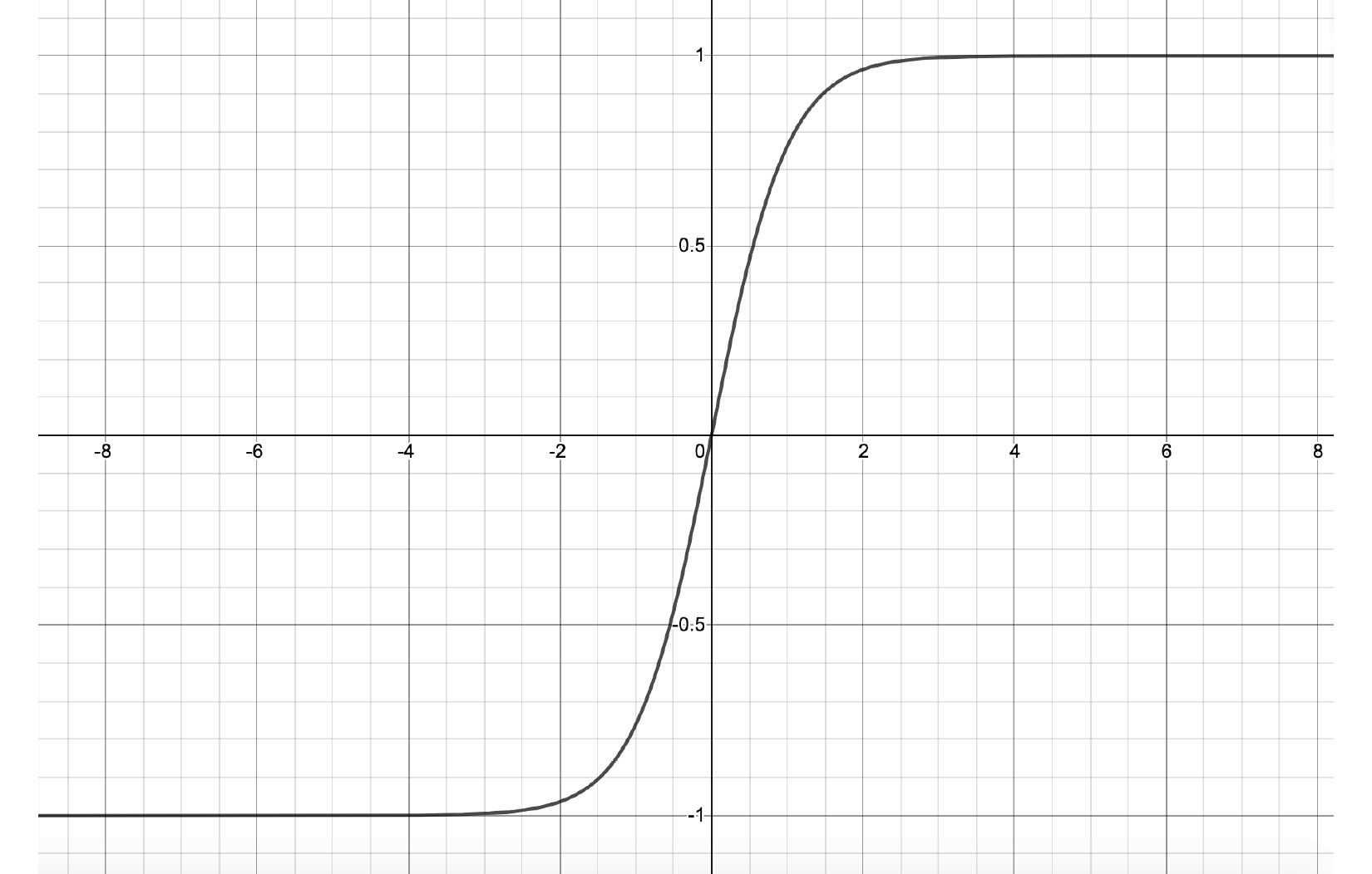
- TanH: TanH is expressed as follows:
The function is shown in graph form as follows:
Figure 1.11 – TanH function
Contrary to sigmoid, the output y varies from -1 to 1 in the case of the TanH activation function. Hence, this activation is useful in cases where we need both positive as well as negative outputs.
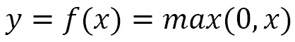
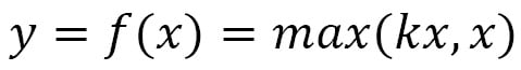
- Rectified linear units (ReLUs): ReLUs are more recent than the previous two and are simply expressed as follows:
The function is shown in graph form as follows:
Figure 1.12 – ReLU function
A distinct feature of ReLU in comparison with the sigmoid and TanH activation functions is that the output keeps growing with the input whenever the input is greater than 0. This prevents the gradient of this function from diminishing to 0 as in the case of the previous two activation functions. Although, whenever the input is negative, both the output and the gradient will be 0.
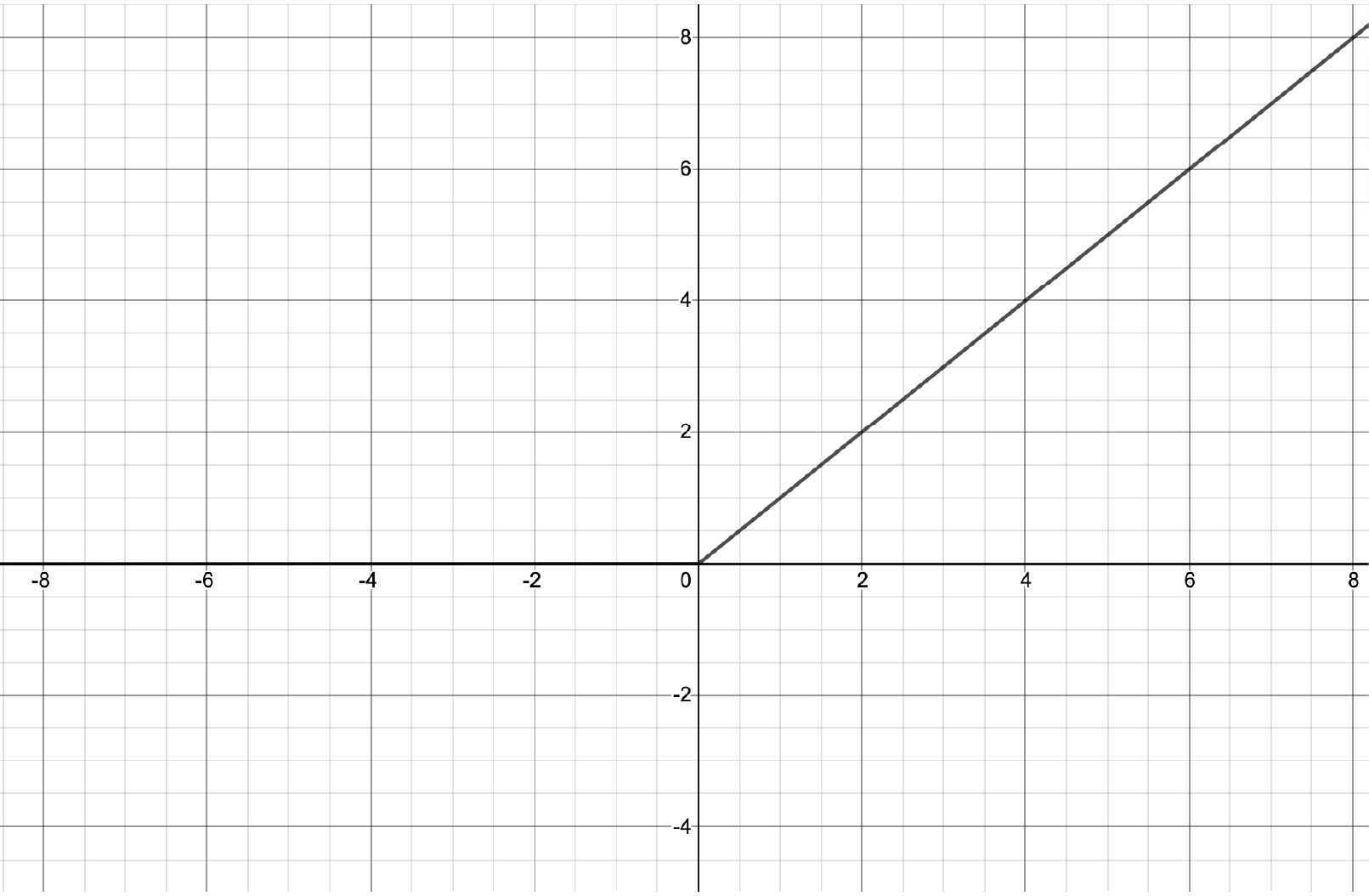
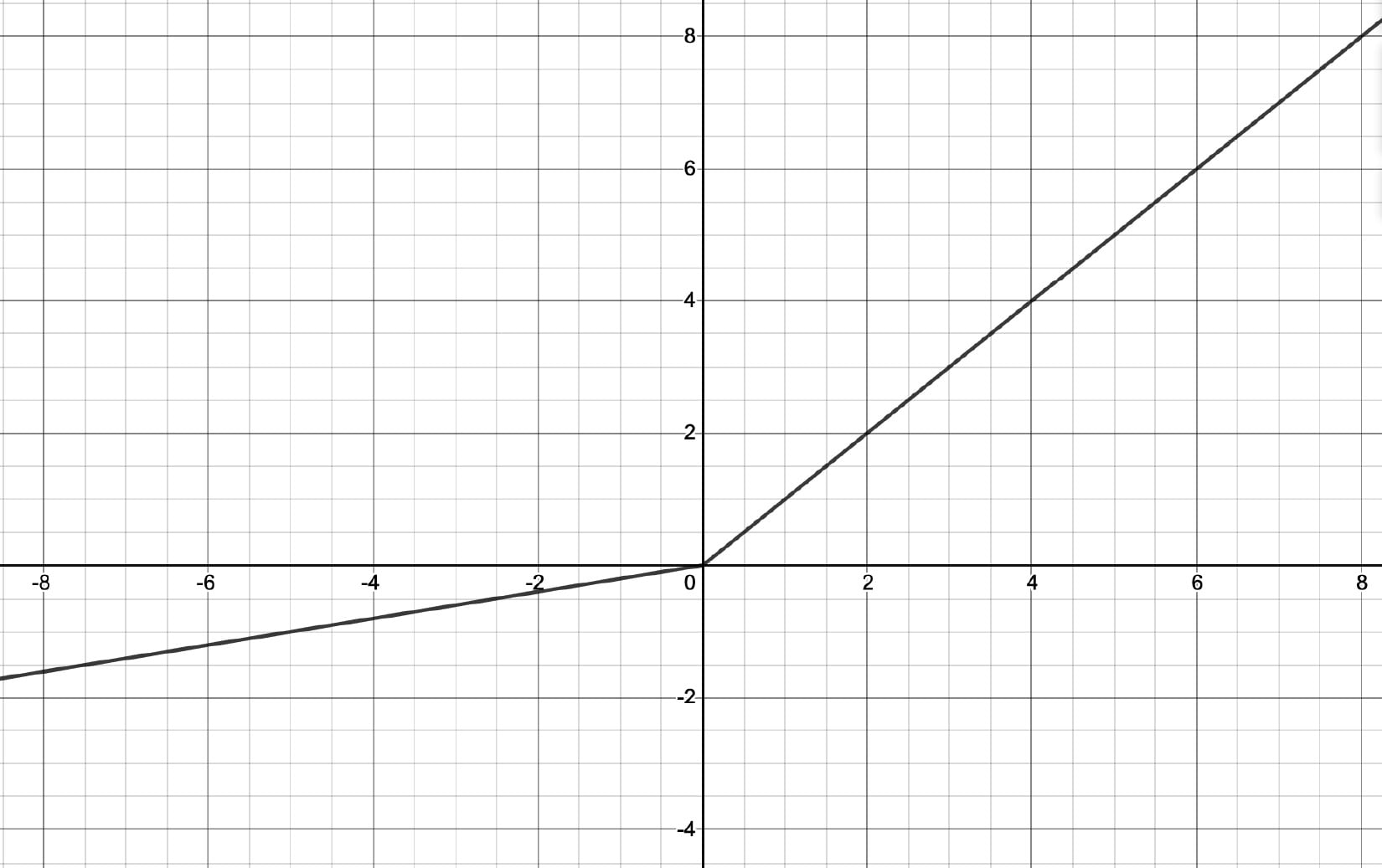
- Leaky ReLU: ReLUs entirely suppress any incoming negative input by outputting 0. We may, however, want to also process negative inputs for some cases. Leaky ReLUs offer the option of processing negative inputs by outputting a fraction k of the incoming negative input. This fraction k is a parameter of this activation function, which can be mathematically expressed as follows:
The following graph shows the input-output relationship for leaky ReLU:
Figure 1.13 – Leaky ReLU function
Activation functions are an actively evolving area of research within deep learning. It will not be possible to list all of the activation functions here but I encourage you to check out the recent developments in this domain. Many activation functions are simply nuanced modifications of the ones mentioned in this section.
Optimization schedule
So far, we have spoken of how a neural network structure is built. In order to train a neural network, we need to adopt an optimization schedule. Like any other parameter-based machine learning model, a deep learning model is trained by tuning its parameters. The parameters are tuned through the process of backpropagation, wherein the final or output layer of the neural network yields a loss. This loss is calculated with the help of a loss function that takes in the neural network's final layer's outputs and the corresponding ground truth target values. This loss is then backpropagated to the previous layers using gradient descent and the chain rule of differentiation.
The parameters or weights at each layer are accordingly modified in order to minimize the loss. The extent of modification is determined by a coefficient, which varies from 0 to 1, also known as the learning rate. This whole procedure of updating the weights of a neural network, which we call the optimization schedule, has a significant impact on how well a model is trained. Therefore, a lot of research has been done in this area and is still ongoing. The following are a few popular optimization schedules:
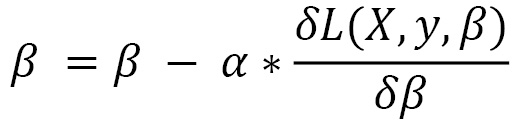
- Stochastic Gradient Descent (SGD): It updates the model parameters in the following fashion:
β is the parameter of the model and X and y are the input training data and the corresponding labels respectively. L is the loss function and α is the learning rate. SGD performs this update for every training example pair (X, y). A variant of this –mini-batch gradient descent – performs updates for every k examples, where k is the batch size. Gradients are calculated altogether for the whole mini-batch. Another variant, batch gradient descent, performs parameter updates by calculating the gradient across the entire dataset.
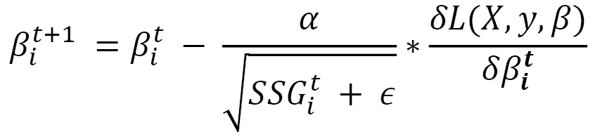
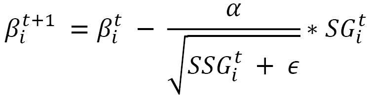
- Adagrad: In the previous optimization schedule, we used a single learning rate for all the parameters of the model. However, different parameters might need to be updated at different paces, especially in cases of sparse data, where some parameters are more actively involved in feature extraction than others. Adagrad introduces the idea of per-parameter updates, as shown here:
Here, we use the subscript i to denote the ith parameter and the superscript t is used to denote the time step t of the gradient descent iterations. SSGit is the sum of squared gradients for the ith parameter starting from time step 0 to time step t. є is used to denote a small value added to SSG to avoid division by zero. Dividing the global learning rate α by the square root of SSG ensures that the learning rate for frequently changing parameters lowers faster than the learning rate for rarely updated parameters.
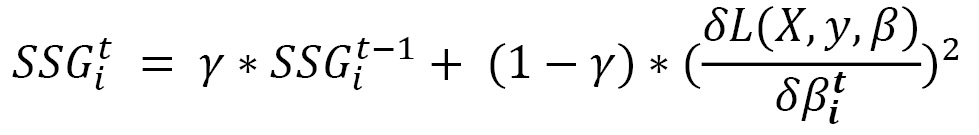
- Adadelta: In Adagrad, the denominator of the learning rate is a term that keeps on rising in value due to added squared terms in every time step. This causes the learning rates to decay to vanishingly small values. To tackle this problem, Adadelta introduces the idea of computing the sum of squared gradients only up to previous time steps. In fact, we can express it as a running decaying average of the past gradients:
γ here is the decaying factor we wish to choose for the previous sum of squared gradients. With this formulation, we ensure that the sum of squared gradients does not accumulate to a large value, thanks to the decaying average. Once SSGit is defined, we can use the Adagrad equation to define the update step for Adadelta.
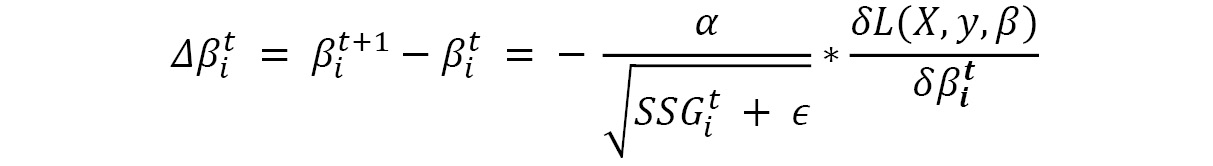
However, if we look closely at the Adagrad equation, the root mean squared gradient is not a dimensionless quantity and hence should ideally not be used as a coefficient for the learning rate. To resolve this, we define another running average, this time for the squared parameter updates. Let's first define the parameter update:
And then, similar to the running decaying average of the past gradients equation (the first equation under Adadelta), we can define the square sum of parameter updates as follows:
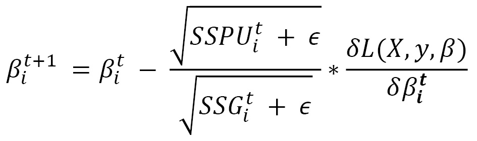
Here, SSPU is the sum of squared parameter updates. Once we have this, we can adjust for the dimensionality problem in the Adagrad equation with the final Adadelta equation:
Noticeably, the final Adadelta equation doesn't require any learning rate. One can still however provide a learning rate as a multiplier. Hence, the only mandatory hyperparameter for this optimization schedule is the decaying factors..
- RMSprop: We have implicitly discussed the internal workings of RMSprop while discussing Adadelta as both are pretty similar. The only difference is that RMSProp does not adjust for the dimensionality problem and hence the update equation stays the same as the equation presented in the Adagrad section, wherein the SSGit is obtained from the first equation in the Adadelta section. This essentially means that we do need to specify both a base learning rate as well as a decaying factor in the case of RMSProp.
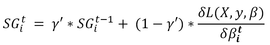
- Adaptive Moment Estimation (Adam): This is another optimization schedule that calculates customized learning rates for each parameter. Just like Adadelta and RMSprop, Adam also uses the decaying average of the previous squared gradients as demonstrated in the first equation in the Adadelta section. However, it also uses the decaying average of previous gradient values:
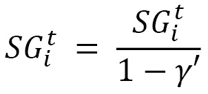
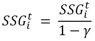
SG and SSG are mathematically equivalent to estimating the first and second moments of the gradient respectively, hence the name of this method – adaptive moment estimation. Usually, γ and γ' are close to 1 and in that case, the initial values for both SG and SSG might be pushed towards zero. To counteract that, these two quantities are reformulated with the help of bias correction:
and
Once they are defined, the parameter update is expressed as follows:
Basically, the gradient on the extreme right-hand side of the equation is replaced by the decaying average of the gradient. Noticeably, Adam optimization involves three hyperparameters – the base learning rate, and the two decaying rates for the gradients and squared gradients. Adam is one of the most successful, if not the most successful, optimization schedule in recent times for training complex deep learning models.
So, which optimizer shall we use? It depends. If we are dealing with sparse data, then the adaptive optimizers (numbers 2 to 5) will be advantageous because of the per-parameter learning rate updates. As mentioned earlier, with sparse data, different parameters might be worked at different paces and hence a customized per-parameter learning rate mechanism can greatly help the model in reaching optimal solutions. SGD might also find a decent solution but will take much longer in terms of training time. Among the adaptive ones, Adagrad has the disadvantage of vanishing learning rates due to a monotonically increasing learning rate denominator.
RMSProp, Adadelta, and Adam are quite close in terms of their performance on various deep learning tasks. RMSprop is largely similar to Adadelta, except for the use of the base learning rate in RMSprop versus the use of the decaying average of previous parameter updates in Adadelta. Adam is slightly different in that it also includes the first-moment calculation of gradients and accounts for bias correction. Overall, Adam could be the optimizer to go with, all else being equal. We will use some of these optimization schedules in the exercises in this book. Feel free to switch them with another one to observe changes in the following:
- Model training time and trajectory (convergence)
- Final model performance
In the coming chapters, we will use many of these architectures, layers, activation functions, and optimization schedules in solving different kinds of machine learning problems with the help of PyTorch. In the example included in this chapter, we will create a convolutional neural network that contains convolutional, linear, max-pooling, and dropout layers. Log-Softmax is used for the final layer and ReLU is used as the activation function for all the other layers. And the model is trained using an Adadelta optimizer with a fixed learning rate of 0.5.


 Free Chapter