Originally, IPython provided an enhanced command-line console to run Python code interactively. The Jupyter Notebook is a more recent and more sophisticated alternative to the console. Today, both tools are available, and we recommend that you learn to use both.
Launching the IPython console
To run the IPython console, type ipython in an OS terminal. There, you can write Python commands and see the results instantly. Here is a screenshot:
The IPython console is most convenient when you have a command-line-based workflow and you want to execute some quick Python commands.
You can exit the IPython console by typing exit.
Note
Let's mention the Qt console, which is similar to the IPython console but offers additional features such as multiline editing, enhanced tab completion, image support, and so on. The Qt console can also be integrated within a graphical application written with Python and Qt. See http://jupyter.org/qtconsole/stable/ for more information.
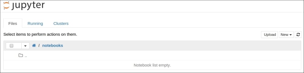
Launching the Jupyter Notebook
To run the Jupyter Notebook, open an OS terminal, go to ~/minibook/ (or into the directory where you've downloaded the book's notebooks), and type jupyter notebook. This will start the Jupyter server and open a new window in your browser (if that's not the case, go to the following URL: http://localhost:8888). Here is a screenshot of Jupyter's entry point, the Notebook dashboard:
Note
At the time of writing, the following browsers are officially supported: Chrome 13 and greater; Safari 5 and greater; and Firefox 6 or greater. Other browsers may work also. Your mileage may vary.
The Notebook is most convenient when you start a complex analysis project that will involve a substantial amount of interactive experimentation with your code. Other common use-cases include keeping track of your interactive session (like a lab notebook), or writing technical documents that involve code, equations, and figures.
In the rest of this section, we will focus on the Notebook interface.
Tip
Closing the Notebook server
To close the Notebook server, go to the OS terminal where you launched the server from, and press Ctrl + C. You may need to confirm with y.
The dashboard contains several tabs:
- Files: shows all files and notebooks in the current directory
- Running: shows all kernels currently running on your computer
- Clusters: lets you launch kernels for parallel computing (covered in Chapter 5, High-Performance and Parallel Computing)
A notebook is an interactive document containing code, text, and other elements. A notebook is saved in a file with the .ipynb extension. This file is a plain text file storing a JSON data structure.
A kernel is a process running an interactive session. When using IPython, this kernel is a Python process. There are kernels in many languages other than Python.
Note
We follow the convention to use the term notebook for a file, and Notebook for the application and the web interface.
In Jupyter, notebooks and kernels are strongly separated. A notebook is a file, whereas a kernel is a process. The kernel receives snippets of code from the Notebook interface, executes them, and sends the outputs and possible errors back to the Notebook interface. Thus, in general, the kernel has no notion of a Notebook. A notebook is persistent (it's a file), whereas a kernel may be closed at the end of an interactive session and it is therefore not persistent. When a notebook is re-opened, it needs to be re-executed.
In general, no more than one Notebook interface can be connected to a given kernel. However, several IPython consoles can be connected to a given kernel.
The Notebook user interface
To create a new notebook, click on the New button, and select Notebook (Python 3). A new browser tab opens and shows the Notebook interface as follows:
Here are the main components of the interface, from top to bottom:
- The notebook name, which you can change by clicking on it. This is also the name of the
.ipynb file. - The Menu bar gives you access to several actions pertaining to either the notebook or the kernel.
- To the right of the menu bar is the Kernel name. You can change the kernel language of your notebook from the Kernel menu. We will see in Chapter 6, Customizing IPython how to manage different kernel languages.
- The Toolbar contains icons for common actions. In particular, the dropdown menu showing Code lets you change the type of a cell.
- Following is the main component of the UI: the actual Notebook. It consists of a linear list of cells. We will detail the structure of a cell in the following sections.
Structure of a notebook cell
There are two main types of cells: Markdown cells and code cells, and they are described as follows:
- A Markdown cell contains rich text. In addition to classic formatting options like bold or italics, we can add links, images, HTML elements, LaTeX mathematical equations, and more. We will cover Markdown in more detail in the Ten Jupyter/IPython essentials section of this chapter.
- A code cell contains code to be executed by the kernel. The programming language corresponds to the kernel's language. We will only use Python in this book, but you can use many other languages.
You can change the type of a cell by first clicking on a cell to select it, and then choosing the cell's type in the toolbar's dropdown menu showing Markdown or Code.
Here is a screenshot of a Markdown cell:
The top panel shows the cell in edit mode, while the bottom one shows it in render mode. The edit mode lets you edit the text, while the render mode lets you display the rendered cell. We will explain the differences between these modes in greater detail in the following section.
Here is a screenshot of a complex code cell:
This code cell contains several parts, as follows:
- The Prompt number shows the cell's number. This number increases every time you run the cell. Since you can run cells of a notebook out of order, nothing guarantees that code numbers are linearly increasing in a given notebook.
- The Input area contains a multiline text editor that lets you write one or several lines of code with syntax highlighting.
- The Widget area may contain graphical controls; here, it displays a slider.
- The Output area can contain multiple outputs, here:
- Standard output (text in black)
- Error output (text with a red background)
- Rich output (an HTML table and an image here)
The Notebook modal interface
The Notebook implements a modal interface similar to some text editors such as vim. Mastering this interface may represent a small learning curve for some users.
- Use the edit mode to write code (the selected cell has a green border, and a pen icon appears at the top right of the interface). Click inside a cell to enable the edit mode for this cell (you need to double-click with Markdown cells).
- Use the command mode to operate on cells (the selected cell has a gray border, and there is no pen icon). Click outside the text area of a cell to enable the command mode (you can also press the Esc key).
Keyboard shortcuts are available in the Notebook interface. Type h to show them. We review here the most common ones (for Windows and Linux; shortcuts for OS X may be slightly different).
Keyboard shortcuts available in both modes
Here are a few keyboard shortcuts that are always available when a cell is selected:
- Ctrl + Enter: run the cell
- Shift + Enter: run the cell and select the cell below
- Alt + Enter: run the cell and insert a new cell below
- Ctrl + S: save the notebook
Keyboard shortcuts available in the edit mode
In the edit mode, you can type code as usual, and you have access to the following keyboard shortcuts:
- Esc: switch to command mode
- Ctrl + Shift + -: split the cell
Keyboard shortcuts available in the command mode
In the command mode, keystrokes are bound to cell operations. Don't write code in command mode or unexpected things will happen! For example, typing dd in command mode will delete the selected cell! Here are some keyboard shortcuts available in command mode:
- Enter: switch to edit mode
- ↑ or k: select the previous cell
- ↓ or j: select the next cell
- y / m: change the cell type to code cell/Markdown cell
- a / b: insert a new cell above/below the current cell
- x / c / v: cut/copy/paste the current cell
- dd: delete the current cell
- z: undo the last delete operation
- Shift + =: merge the cell below
- h: display the help menu with the list of keyboard shortcuts
Spending some time learning these shortcuts is highly recommended.
Here are a few references:


 Free Chapter