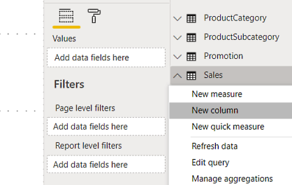
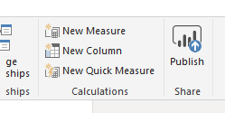
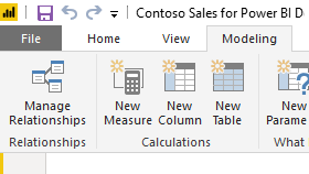
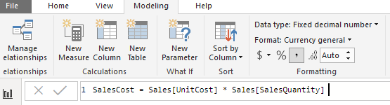
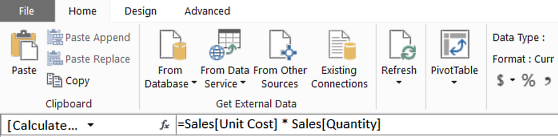
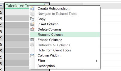
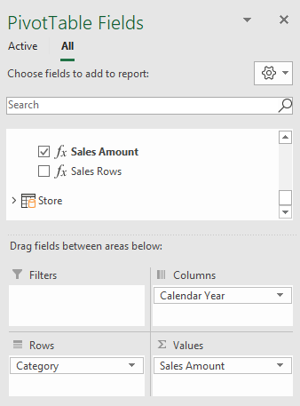
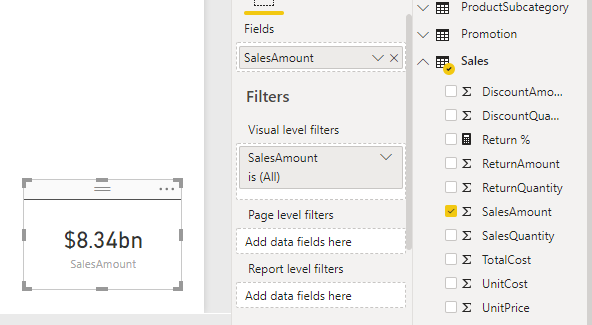
Understanding the difference between a calculated column and a measure (also known as a calculated field) is an important concept that you will need to learn to begin mastering DAX. At first, they may seem very similar, and indeed there are some instances where both can be used to obtain the same result. However, they are different and serve different purposes. Likewise, they also impact resources in different ways. Calculated columns allow you to extend a table in your data model by creating additional columns. Measures allow you to aggregate the values of rows in a table and take into account any current filters or slicers that are applied.

You can create new columns by using DAX expressions if you want to extend a table in your Power BI, Excel Power Pivot, or Analysis Services Tabular data model. These are referred to as calculated columns. In Excel, each row of a column in a worksheet can be defined by using a different expression. However, calculated columns evaluate the same expression throughout the column of a table, calculating the appropriate value on a row-by-row basis.

To create a new calculated column in Power BI Desktop, follow these steps:

1. Start on the report page and highlight the table that you want to add a new column to from the list of tables shown in the Fields pane on the right-hand side.
2. Right-click on the table name and select New column from the menu, as shown in Figure 1-1:

Alternatively, you can highlight the table and click on the New Column button on the Calculations section of the Home ribbon or the Calculations section of the Modeling ribbon, as shown in Figure 1-2:

Or you can highlight the table and click on the New Column button on the Calculations section of the Modeling ribbon, as shown in Figure 1-3:

3. Open the formula editor, and enter the DAX expression that will define your New Column. Figure 1-4 shows the formula editor in Power BI Desktop:

To create a new column in Excel Power Pivot and Analysis Services, we do the following:

1. Go into your data model and select the table you want to add the new column to.
2. Select a cell in the last column labeled Add Column.

3. In the formula editor, write the expression that defines your new column. Figure 1-5 shows the formula editor in Excel. Unlike Power BI, in Excel Power Pivot and Analysis Services, the DAX expression begins with the assignment symbol (=) and not the column name:

4. To rename a new column, once you have entered the expression, right-click on the column name and select Rename Column from the menu, as shown in Figure 1-6:

Calculated columns are computed during a data refresh and stored in memory with the rest of your data model. This is an important point to note when you are planning and building your data model. On the one hand, with complex expressions, the time taken to compute them is at the point you refresh the data and not when you are querying the data. This can improve the user experience, especially with complex expressions, but you need to remember that each calculated column will take up space in memory. Although this might not be an issue with a smaller table, it could have a significant impact on memory use when you are dealing with large tables. If you have complex expressions behind your calculated columns, then this could also slow down the time it takes to refresh the data in your data model.

You would be well advised not to have too many calculated columns in your data model and to consider whether it would be possible to use a measure instead, especially if it does not impact the user experience too adversely.

The other way you can extend your data model is by using measures (also referred to as calculated fields in Excel 2013). Unlike calculated columns, which are evaluated row by row using the context of the current row, measures are used to summarize data by aggregating the values of rows in a table. They work within the current filter context, which means they are affected by the current filters, slicers applied, and the highlighted sections of charts or visuals.

There are two types of measures: implicit and explicit. Implicit measures are created behind the scenes when you drag a field to the Values area of the PivotTable Fields list, as shown in Figure 1-7:

They are also created when you drag a visual on to the desktop of Power BI, as shown in Figure 1-8:

An explicit measure, on the other hand, is a measure that is specifically created by you.

A measure must be created if you want to conduct an operation on aggregate values instead of values on a row-by-row basis. For example, if you need to calculate the percentage ratio of two columns, you will need to create a measure that calculates the ratio based on the sum of each column. The following measure calculates the percentage of returns to sales by dividing the sum of items returned by the sum of items sold:

Return % = 
DIVIDE (
    SUM ( Sales[ReturnQuantity] ), 
    SUM ( Sales[SalesQuantity] )
)

Measures are calculated once for everywhere they are used in a report. They are re-calculated every time a report page loads or a user changes a filter or slicer or highlights part of a chart:

In Figure 1-9, a measure is used to calculate the number of returns over the number of sales. This is used for the value in the column chart, with the sales channel used for the axis. In this example, the measure is calculated four times, once for each time the filter context changes to reflect each of the four different stores.

To create a new measure in Power BI Desktop, follow these steps:

1. Start on the report page and highlight the table that you want to add the new measure to, from the list of tables shown in the Fields pane on the right-hand side.
2. Next, right-click on the table name and select New measure from the menu, as shown in Figure 1-10:

To create a new measure in Excel Power Pivot and Analysis Services, we do the following:

1. Go into your data model and select the table you want to add the measure to.
2. Select a blank cell in the calculation area.
3. In the formula editor, write the expression that defines your new measure. Figure 1-11 shows a couple of measures in the calculation area of an Excel table:

The syntax used to create a measure differs slightly depending on the tool you are using. With Power BI, you use the = assignment operator, whereas with Excel and Analysis Services, you use the := assignment operator. If you use the := assignment operator in Power BI, it will automatically be converted into the = operator.

So, for example, Figure 1-12 shows an example of the syntax used to create a measure in Power BI Desktop:

On the other hand, Figure 1-13 shows an example of the syntax used to create a similar measure in Excel:

Although DAX requires measures to be defined within a table, they can be moved between tables without affecting their functionality. In fact, it is good practice to keep general measures under one table with a name such as Key Measures.

Although they may look similar, calculated columns and measures operate very differently. They both use DAX expressions, but they differ in the point at which they are calculated and in the context of their evaluation:

• The values of calculated columns are calculated during a data refresh and they are evaluated using the current row context. They also take up memory and disk space and can slow down data loading times during data refreshes. However, once loaded, they do not impact performance.
• A measure is executed every time a value uses it in a report or chart. Measures are re-calculated every time a page loads. They are also re-calculated when filters or slicers are changed or a user highlights different parts of a chart or visual. A measure does not add to the space used by a data model, but it may impact the speed of user interactions. Measures operate on aggregates that are defined by the current filter context.

You will need to use a calculated column whenever you want to do the following:

• Use the value in a slicer.
• Use the value in rows or columns of a pivot table.
• Use the value on the axes of a chart.
• Use the value as a filter condition in a DAX query.
• Define an expression that is bound to the current row.

You will need to define a measure whenever you want to do the following:

• Use a value that reflects a user's selection of filters, slicers, or highlighted visuals.
• Calculate a ratio.
• Calculate a percentage.

It is sometimes possible to calculate the same value using either a calculated column or a measure, using different DAX expressions. In most cases, where this is possible, you should use a measure, as this will not increase the size of your data model and use extra memory or disk space. This is especially important if you are working with a table that contains a large number of records.

When naming measures, you should not include the table name in the measure name. Although a measure is created under a table, it does not strictly belong to that table. If you do not include the table name, it can easily be moved between tables if necessary. It also makes it easier to identify as a measure. On the other hand, calculated columns should include the table name.