-
Book Overview & Buying
-
Table Of Contents

-
Feedback & Rating

Quantum Machine Learning and Optimisation in Finance
By :
Quantum Machine Learning and Optimisation in Finance
By:
Overview of this book
With recent advances in quantum computing technology, we finally reached the era of Noisy Intermediate-Scale Quantum (NISQ) computing. NISQ-era quantum computers are powerful enough to test quantum computing algorithms and solve hard real-world problems faster than classical hardware.
Speedup is so important in financial applications, ranging from analysing huge amounts of customer data to high frequency trading. This is where quantum computing can give you the edge. Quantum Machine Learning and Optimisation in Finance shows you how to create hybrid quantum-classical machine learning and optimisation models that can harness the power of NISQ hardware.
This book will take you through the real-world productive applications of quantum computing. The book explores the main quantum computing algorithms implementable on existing NISQ devices and highlights a range of financial applications that can benefit from this new quantum computing paradigm.
This book will help you be one of the first in the finance industry to use quantum machine learning models to solve classically hard real-world problems. We may have moved past the point of quantum computing supremacy, but our quest for establishing quantum computing advantage has just begun!
Table of Contents (4 chapters)
Preface

 Free Chapter
Chapter 1: The Principles of Quantum Mechanics
Part I: Analog Quantum Computing – Quantum Annealing
Part II: Gate Model Quantum Computing
Customer Reviews


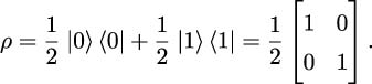
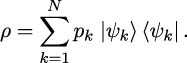
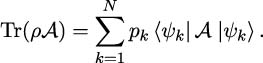
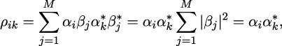
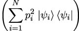
 is a quantum state whose wavefunction is known with certainty (although this does not necessarily provide full knowledge of the measurement statistics), and each p
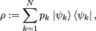
 equals
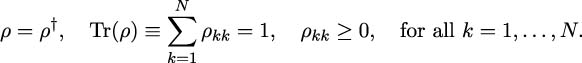
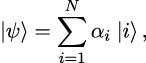

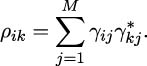
 and therefore ρ


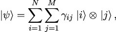
 given by (
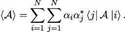
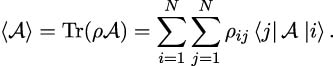
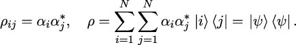
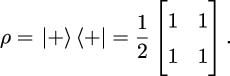


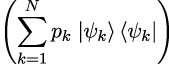

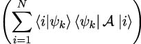
 .
.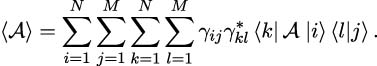
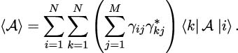


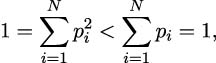


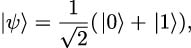
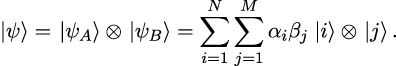
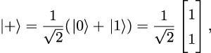
 and
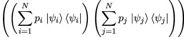
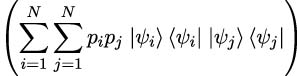
and  . If a physical system is prepared to be either in state
  or state
  with equal probability, it can be described by the mixed state