


In this recipe, the aim of the problem is to predict house prices in Ames, Iowa, given 81 features describing the house, area, land, infrastructure, utilities, and much more. The Ames dataset has a nice combination of categorical and continuous features, a good size, and, perhaps most importantly, it doesn't suffer from problems of potential redlining or data entry like other, similar datasets, such as Boston Housing. We'll concentrate on the main aspects of PyTorch modeling here. We'll do online learning, analogous to Keras, in the Modeling and predicting in Keras recipe in Chapter 1, Getting Started with Artificial Intelligence in Python. If you want to see more details on some of the steps, please look at our notebook on GitHub.
As a little extra, we will also demonstrate neuron importance for the models developed in PyTorch. You can try out different network architectures in PyTorch or model types. The focus in this recipe is on the methodology, not an exhaustive search for the best solution.
Getting ready
In order to prepare for the recipe, we need to do a few things. We'll download the data as in the previous recipe, Transforming data in scikit-learn, and perform some preprocessing by following these steps:
from sklearn.datasets import fetch_openml
data = fetch_openml(data_id=42165, as_frame=True)
You can see the full dataset description at OpenML: https://www.openml.org/d/42165.
Let's look at the features:
import pandas as pd
data_ames = pd.DataFrame(data.data, columns=data.feature_names)
data_ames['SalePrice'] = data.target
data_ames.info()
Here is the DataFrame information:
PyTorch and seaborn are installed by default in Colab. We will assume, even if you are working with your self-hosted install by now, that you'll have the libraries installed.
We'll use one more library, however, captum, which allows the inspection of PyTorch models for feature and neuron importance:
!pip install captum
There is one more thing. We'll assume you have a GPU available. If you don't have a GPU in your computer, we'd recommend you try this recipe on Colab. In Colab, you'll have to choose a runtime type with GPU.
After all these preparations, let's see how we can predict house prices.
How to do it...
The Ames Housing dataset is a small- to mid-sized dataset (1,460 rows) with 81 features, both categorical and numerical. There are no missing values.
In the Keras recipe previously, we've seen how to scale the variables. Scaling is important here because all variables have different scales. Categorical variables need to be converted to numerical types in order to feed them into our model. We have the choice of one-hot encoding, where we create dummy variables for each categorical factor, or ordinal encoding, where we number all factors and replace the strings with these numbers. We could feed the dummy variables in like any other float variable, while ordinal encoding would require the use of embeddings, linear neural network projections that re-order the categories in a multi-dimensional space.
We take the embedding route here:
import numpy as np
from category_encoders.ordinal import OrdinalEncoder
from sklearn.preprocessing import StandardScaler

num_cols = list(data_ames.select_dtypes(include='float'))
cat_cols = list(data_ames.select_dtypes(include='object'))

ordinal_encoder = OrdinalEncoder().fit(
    data_ames[cat_cols]
)
standard_scaler = StandardScaler().fit(
    data_ames[num_cols]
)

X = pd.DataFrame(
    data=np.column_stack([
        ordinal_encoder.transform(data_ames[cat_cols]),
        standard_scaler.transform(data_ames[num_cols])
    ]),
    columns=cat_cols + num_cols
)
We go through the data analysis, such as correlation and distribution plots, in a lot more detail in the notebook on GitHub.
Now we can split the data into training and test sets, as we did in previous recipes. Here, we add a stratification of the numerical variable. This makes sure that different sections (five of them) are included at equal measure in both training and test sets:
np.random.seed(12)
from sklearn.model_selection import train_test_split

bins = 5
sale_price_bins = pd.qcut(
    X['SalePrice'], q=bins, labels=list(range(bins))
)
X_train, X_test, y_train, y_test = train_test_split(
    X.drop(columns='SalePrice'),
    X['SalePrice'],
    random_state=12,
    stratify=sale_price_bins
)
Before going ahead, let's look at the importance of the features using a model-independent technique.
Before we run anything, however, let's make sure we are running on the GPU:
device = torch.device('cuda')
torch.backends.cudnn.benchmark = True
Let's build our PyTorch model, similar to the Classifying in scikit-learn, Keras, and PyTorch recipe in Chapter 1, Getting Started with Artificial Intelligence in Python.
We'll implement a neural network regression with batch inputs using PyTorch. This will involve the following steps:
- Converting data to torch tensors
- Defining the model architecture
- Defining the loss criterion and optimizer
- Creating a data loader for batches
- Running the training
Without further preamble, let's get to it:
- Begin by converting the data to torch tensors:
from torch.autograd import Variable

num_features = list(
    set(num_cols) - set(['SalePrice', 'Id'])
)
X_train_num_pt = Variable(
    torch.cuda.FloatTensor(
        X_train[num_features].values
    )
)
X_train_cat_pt = Variable(
    torch.cuda.LongTensor(
        X_train[cat_cols].values
    )
)
y_train_pt = Variable(
    torch.cuda.FloatTensor(y_train.values)
).view(-1, 1)
X_test_num_pt = Variable(
    torch.cuda.FloatTensor(
        X_test[num_features].values
    )
)
X_test_cat_pt = Variable(
   torch.cuda.LongTensor(
        X_test[cat_cols].values
    ).long()
)
y_test_pt = Variable(
    torch.cuda.FloatTensor(y_test.values)
).view(-1, 1)
This makes sure we load our numerical and categorical data into separate variables, similar to NumPy. If you mix data types in a single variable (array/matrix), they'll become objects. We want to get our numerical variables as floats, and the categorical variables as long (or int) indexing our categories. We also separate the training and test sets.
Clearly, an ID variable should not be important in a model. In the worst case, it could introduce a target leak if there's any correlation of the ID with the target. We've removed it from further processing.
- Define the model architecture:
class RegressionModel(torch.nn.Module):

    def __init__(self, X, num_cols, cat_cols, device=torch.device('cuda'), embed_dim=2, hidden_layer_dim=2, p=0.5):
        super(RegressionModel, self).__init__()
        self.num_cols = num_cols
        self.cat_cols = cat_cols
        self.embed_dim = embed_dim
        self.hidden_layer_dim = hidden_layer_dim

        self.embeddings = [
            torch.nn.Embedding(
                num_embeddings=len(X[col].unique()),
                embedding_dim=embed_dim
            ).to(device)
            for col in cat_cols
        ]
        hidden_dim = len(num_cols) + len(cat_cols) * embed_dim,

        # hidden layer
        self.hidden = torch.nn.Linear(torch.IntTensor(hidden_dim), hidden_layer_dim).to(device)
        self.dropout_layer = torch.nn.Dropout(p=p).to(device)
        self.hidden_act = torch.nn.ReLU().to(device)

        # output layer
        self.output = torch.nn.Linear(hidden_layer_dim, 1).to(device)

    def forward(self, num_inputs, cat_inputs):
        '''Forward method with two input variables -
        numeric and categorical.
        '''
        cat_x = [
            torch.squeeze(embed(cat_inputs[:, i] - 1))
            for i, embed in enumerate(self.embeddings)
        ]
        x = torch.cat(cat_x + [num_inputs], dim=1)
        x = self.hidden(x)
        x = self.dropout_layer(x)
        x = self.hidden_act(x)
        y_pred = self.output(x)
        return y_pred

house_model = RegressionModel(
    data_ames, num_features, cat_cols
)
Our activation function on the two linear layers (dense layers, in Keras terminology) is the rectified linear unit activation (ReLU) function. Please note that we couldn't have encapsulated the same architecture (easily) as a sequential model because of the different operations occurring on categorical and numerical types.
- Next, define the loss criterion and optimizer. We take the mean square error (MSE) as the loss and stochastic gradient descent as our optimization algorithm:
criterion = torch.nn.MSELoss().to(device)
optimizer = torch.optim.SGD(house_model.parameters(), lr=0.001)
- Now, create a data loader to input a batch of data at a time:
data_batch = torch.utils.data.TensorDataset(
    X_train_num_pt, X_train_cat_pt, y_train_pt
)
dataloader = torch.utils.data.DataLoader(
    data_batch, batch_size=10, shuffle=True
)
We set a batch size of 10. Now we can do our training.
- Run the training!
Since this seems so much more verbose than what we saw in Keras in the Classifying in scikit-learn, Keras, and PyTorch recipe in Chapter 1, Getting Started with Artificial Intelligence in Python, we commented this code quite heavily. Basically, we have to loop over epochs, and within each epoch an inference is performance, an error is calculated, and the optimizer applies the adjustments according to the error.
This is the loop over epochs without the inner loop for training:
from tqdm.notebook import trange

train_losses, test_losses = [], []
n_epochs = 30
for epoch in trange(n_epochs):
    train_loss, test_loss = 0, 0
    # training code will go here:
    # <...>

    # print the errors in training and test:
    if epoch % 10 == 0 :
        print(
            'Epoch: {}/{}\t'.format(epoch, 1000),
            'Training Loss: {:.3f}\t'.format(
                train_loss / len(dataloader)
            ),
            'Test Loss: {:.3f}'.format(
                test_loss / len(dataloader)
            )
        )
The training is performed inside this loop over all the batches of the training data. This looks as follows:
    for (x_train_num_batch,
         x_train_cat_batch,
         y_train_batch) in dataloader:
        # predict y by passing x to the model
        (x_train_num_batch,
         x_train_cat_batch, y_train_batch) = (
                x_train_num_batch.to(device),
                x_train_cat_batch.to(device),
                y_train_batch.to(device)
        )
        pred_ytrain = house_model.forward(
            x_train_num_batch, x_train_cat_batch
        )
        # calculate and print loss:
        loss = torch.sqrt(
            criterion(pred_ytrain, y_train_batch)
        )

        # zero gradients, perform a backward pass,
        # and update the weights.
        optimizer.zero_grad()
        loss.backward()
        optimizer.step()
        train_loss += loss.item()
        with torch.no_grad():
            house_model.eval()
            pred_ytest = house_model.forward(
                X_test_num_pt, X_test_cat_pt
            )
            test_loss += torch.sqrt(
                criterion(pred_ytest, y_test_pt)
            )

        train_losses.append(train_loss / len(dataloader))
        test_losses.append(test_loss / len(dataloader))
This is the output we get. TQDM provides us with a helpful progress bar. At every tenth epoch, we print an update to show training and validation performance:
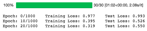
Please note that we take the square root of nn.MSELoss because nn.MSELoss in PyTorch is defined as follows:
((input-target)**2).mean()
Let's plot how our model performs for training and validation datasets during training:
plt.plot(
    np.array(train_losses).reshape((n_epochs, -1)).mean(axis=1),
    label='Training loss'
)
plt.plot(
    np.array(test_losses).reshape((n_epochs, -1)).mean(axis=1),
    label='Validation loss'
)
plt.legend(frameon=False)
plt.xlabel('epochs')
plt.ylabel('MSE')
The following diagram shows the resulting plot:
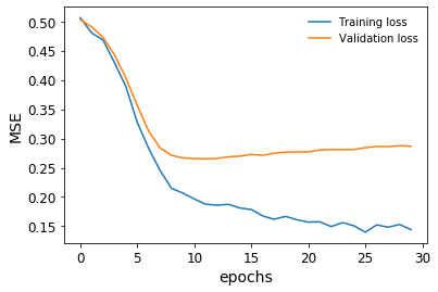
We stopped our training just in time before our validation loss stopped decreasing.
We can also rank and bin our target variable and plot the predictions against it in order to see how the model is performing across the whole spectrum of house prices. This is to avoid the situation in regression, especially with MSE as the loss, that you only predict well for a mid-range of values, close to the mean, but don't do well for anything else. You can find the code for this in the notebook on GitHub. This is called a lift chart (here with 10 bins):
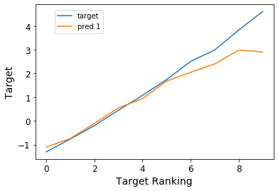
We can see that the model, in fact, predicts very closely across the whole range of house prices. In fact, we get a Spearman rank correlation of about 93% with very high significance, which confirms that this model performs with high accuracy.
How it works...
The deep learning neural network frameworks use different optimization algorithms. Popular among them are Stochastic Gradient Descent (SGD), Root Mean Square Propogation (RMSProp), and Adaptive Moment Estimation (ADAM).
We defined stochastic gradient descent as our optimization algorithm. Alternatively, we could have defined other optimizers:
opt_SGD = torch.optim.SGD(net_SGD.parameters(), lr=LR)
opt_Momentum = torch.optim.SGD(net_Momentum.parameters(), lr=LR, momentum=0.6)
opt_RMSprop = torch.optim.RMSprop(net_RMSprop.parameters(), lr=LR, alpha=0.1)
opt_Adam = torch.optim.Adam(net_Adam.parameters(), lr=LR, betas=(0.8, 0.98))
SGD works the same as gradient descent except that it works on a single example at a time. The interesting part is that the convergence is similar to the gradient descent and is easier on the computer memory.
RMSProp works by adapting the learning rates of the algorithm according to the gradient signs. The simplest of the variants checks the last two gradient signs and then adapts the learning rate by increasing it by a fraction if they are the same, or decreases it by a fraction if they are different.
ADAM is one of the most popular optimizers. It's an adaptive learning algorithm that changes the learning rate according to the first and second moments of the gradients.
Captum is a tool that can help us understand the ins and outs of the neural network model learned on the datasets. It can assist in learning the following:
- Feature importance
- Layer importance
- Neuron importance
This is very important in learning interpretable neural networks. Here, integrated gradients have been applied to understand feature importance. Later, neuron importance is also demonstrated by using the layer conductance method.
There's more...
Given that we have our neural network defined and trained, let's find the important features and neurons using the captum library:
from captum.attr import (
    IntegratedGradients,
    LayerConductance,
    NeuronConductance
)
house_model.cpu()
for embedding in house_model.embeddings:
    embedding.cpu()

house_model.cpu()
ing_house = IntegratedGradients(forward_func=house_model.forward, )
#X_test_cat_pt.requires_grad_()
X_test_num_pt.requires_grad_()
attr, delta = ing_house.attribute(
 X_test_num_pt.cpu(),
 target=None,
 return_convergence_delta=True,
 additional_forward_args=X_test_cat_pt.cpu()
)
attr = attr.detach().numpy()
Now, we have a NumPy array of feature importances.
Layer and neuron importance can also be obtained using this tool. Let's look at the neuron importances of our first layer. We can pass on house_model.act1, which is the ReLU activation function on top of the first linear layer:
cond_layer1 = LayerConductance(house_model, house_model.act1)
cond_vals = cond_layer1.attribute(X_test, target=None)
cond_vals = cond_vals.detach().numpy()
df_neuron = pd.DataFrame(data = np.mean(cond_vals, axis=0), columns=['Neuron Importance'])
df_neuron['Neuron'] = range(10)
This is how it looks:
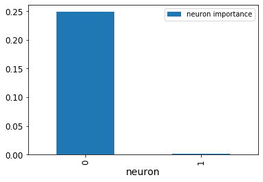
The diagram shows the neuron importances. Apparently, one neuron is just not important.
We can also see the most important variables by sorting the NumPy array we've obtained earlier:
df_feat = pd.DataFrame(np.mean(attr, axis=0), columns=['feature importance'] )
df_feat['features'] = num_features
df_feat.sort_values(
    by='feature importance', ascending=False
).head(10)
So here's a list of the 10 most important variables:
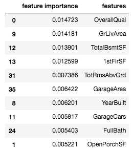
Often, feature importances can help us to both understand the model and prune our model to become less complex (and hopefully less overfitted).
See also
The PyTorch documentation includes everything you need to know about layer types, data loading, losses, metrics, and training: https://pytorch.org/docs/stable/nn.html
A detailed discussion about optimization algorithms can be found in the following article: https://imaddabbura.github.io/post/gradient-descent-algorithm/. Geoffrey Hinton and others explain mini-batch gradient descent in a presentation slide deck: https://www.cs.toronto.edu/~tijmen/csc321/slides/lecture_slides_lec6.pdf. Finally, you can find all the details on ADAM in the article that introduced it: https://arxiv.org/abs/1412.6980.
Captum provides a lot of functionality as regards the interpretability and model inspection of PyTorch models. It's worth having a look at its comprehensive documentation at https://captum.ai/. Details can be found in the original paper at https://arxiv.org/pdf/1703.01365.pdf.


