Detecting stationarity

Stationarity is a central concept in time series analysis and an important assumption made by many time series models. This recipe walks you through the process of testing a time series for stationarity.

Getting ready

A time series is stationary if its statistical properties do not change. It does not mean that the series does not change over time, just that the way it changes does not itself change over time. This includes the level of the time series, which is constant under stationary conditions. Time series patterns such as trend or seasonality break stationarity. Therefore, it may help to deal with these issues before modeling. As we described in the Decomposing a time series recipe, there is evidence that removing seasonality improves the forecasts of deep learning models.

We can stabilize the mean level of the time series by differencing. Differencing is the process of taking the difference between consecutive observations. This process works in two steps:

1. Estimate the number of differencing steps required for stationarity.
2. Apply the required number of differencing operations.

How to do it…

We can estimate the required differencing steps with statistical tests, such as the augmented Dickey-Fuller test, or the KPSS test. These are implemented in the ndiffs() function, which is available in the pmdarima library:

from pmdarima.arima import ndiffs
ndiffs(x=series_daily, test='adf')

Besides the time series, we pass test='adf' as an input to set the method to the augmented Dickey-Fuller test. The output of this function is the number of differencing steps, which in this case is 1. Then, we can differentiate the time series using the diff() method:

series_changes = series_daily.diff()

Differencing can also be applied over seasonal periods. In such cases, seasonal differencing involves computing the difference between consecutive observations of the same seasonal period:

from pmdarima.arima import nsdiffs
nsdiffs(x=series_changes, test='ch', m=365)

Besides the data and the test (ch for Canova-Hansen), we also specify the number of periods. In this case, this parameter is set to 365 (number of days in a year).

How it works…

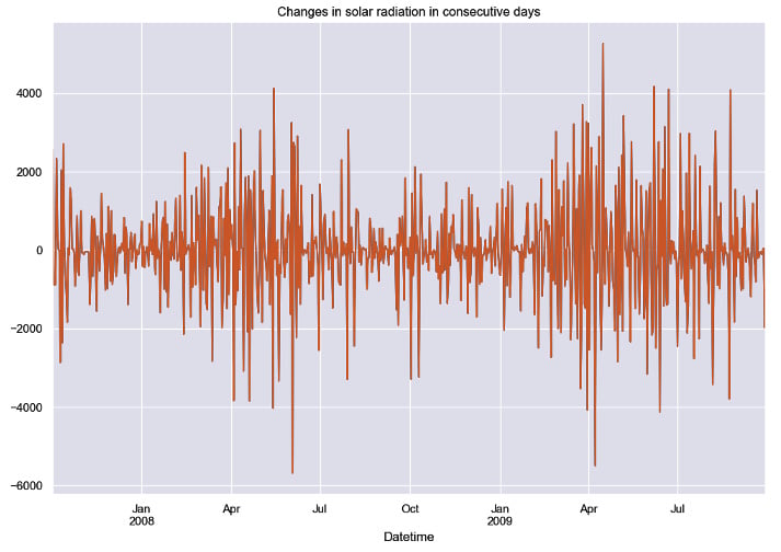
The differenced time series is shown in the following figure.

Figure 1.5: Sample of the series of changes between consecutive periods after differencing

Differencing works as a preprocessing step. First, the time series is differenced until it becomes stationary. Then, a forecasting model is created based on the differenced time series. The forecasts provided by the model can be transformed to the original scale by reverting the differencing operations.

There’s more…

In this recipe, we focused on two particular methods for testing stationarity. You can check other options in the function documentation: https://alkaline-ml.com/pmdarima/modules/generated/pmdarima.arima.ndiffs.html.